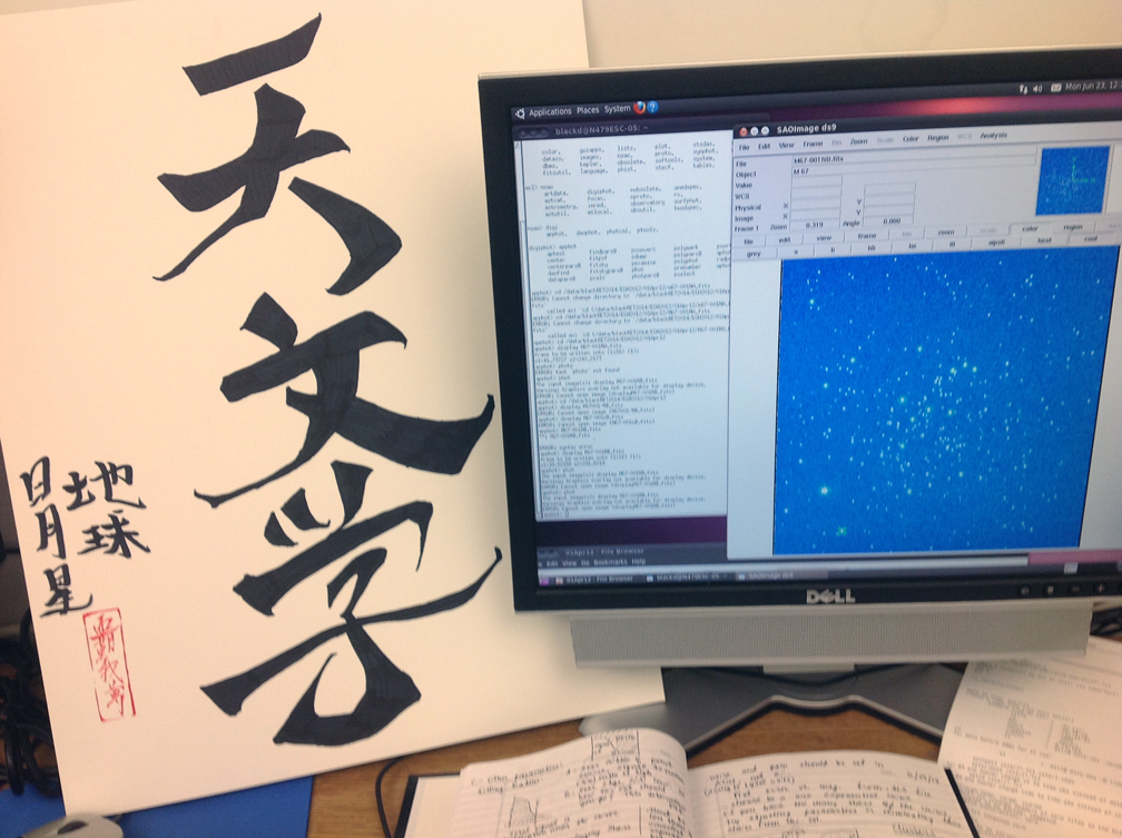
Computer terminal with IRAF and DS9 software running.

For my first two weeks at BYU, I have essentially been in background research mode between preparing my Prospectus and learning how to use IRAF. I hope to eventually work through the process of applying the calibration frames (zeros, darks, and flats) to reduce an image for photometry, but for now the data I am using has already been processed. For this third week, I began to actually analyze the images and pull useful data from them using a software package in IRAF called DAOphot. It was developed by Peter Stetson of the Dominion Astrophysical Observatory in Victoria, British Columbia, Canada.

Coordinates file for NGC 663 in IRAF and DS9.

The purpose of DAOphot is to do photometry (measuring the relative brightness of stars) in crowded clusters. If one is looking an individual stars in a sparse field, then regular aperture photometry works well enough. But stars in a crowded field such as a young open cluster will be hard to separate from each other. Their light curves will overlap. Some stars may be so bright in an image that the CCD sensors become saturated. DAOphot has the ability to separate out the different stars, repair their light curves using a point spread function, and interpolate the results.

Moving through the levels of IRAF – first NOAO, then Digiphot, then DAOphot.

Again, an analogy might help. Seven years ago my students and I filmed and edited a 2-hour documentary on the history of AM radio in Utah. We used a panel format to interview 25 current and former DJs about what it was like working at Utah’s stations. We used whatever microphones and cameras we could scrounge, and we had well over 20 hours of footage by the time the interviews were done. Then came the fun part – editing it all down to two hours. We also soon realized that we hadn’t done a great job of placing the microphones – some of the audio was too loud and the waveforms all had plateaus on top, meaning the sound had maxed out or saturated the microphones.

We were fortunate to have Mike Wizland help us on the project. He’s an expert on audio restoration and teaches at Utah Valley University. He has designed algorithms (as compared with Al Gore Rhythms) that will reconstruct the missing top of the waveform, as well as separate out overlapping speech, where two DJs were talking at once. They call him The Wiz for good reason.

DAOphot does much the same for stars. It digitally reconstructs the light curves. But it requires setting up quite a few parameters to make the point spread function work and extract the stellar magnitudes. Here’s how it works:

Using the IMEXAM command to determine parameters such as FWHM in NGC663.

Step 1: Determining Parameters

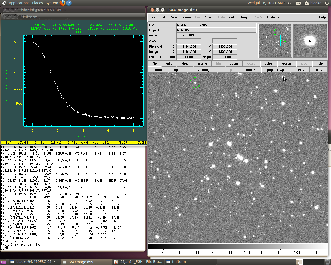
To get the right results, a series of parameters must be determined and set in DAOphot. I first open up IRAF and DS9, then load in the desired frame of the object I’m looking at, such as NGC 663 or NGC 659. Once that’s ready, I use the IMEXAM command in DAOphot to measure four numbers which will set up the point spread function. To explain, I have to talk about one of the big problems with astronomy, namely light scattering.

All the stars, even the close ones, are so far away that to all extents and purposes they should appear as perfect dimensionless points to our eyes. However, the light from these points is scattered as it passes through interstellar dust and our own atmosphere. If the star is near ecliptic, zodiacal dust (dust in our own solar system) will scatter it even more. Since blue light gets scattered more easily than red (which is why the sky is blue, by the way), the light from distant objects becomes more reddish.

We can correct for the reddening, but the scattering spreads our nice one-dimensional perfect points into a smeared out three-dimensional Gaussian curve. If the stars are overlapping, so does the curve. How focused the curve is (or how bad the scattering) will change from night to night depending on seeing conditions. So we have to load in an image from each night and figure out how good the conditions were.

Finding the High Good Datum and the Point Spread Function Radius in DAOphot.

In IMEXAM a black circle appears in DS9. You start by measuring how spread out the light is by hovering over the exact center of 10 or so stars and pressing the “A” key. A series of numbers appears in IRAF. The column labeled “Enclosed” provides the FWHM, or Full-Width at Half Maximum. This refers to the spread of the Gaussian curve, or how wide the light is spread out, at the point that is half of the brightest value at the center of the star (the half maximum). After doing a sampling of stars, both bright and normal, you take the average of the FWHM measures.

Next, you hover over ten or so areas of background, where there are no stars as far as you can tell. This area should be perfectly black but usually is not. You press the “M” key, and another set of numbers appears. This is the standard deviation of the background, called sigma, and represents the error or divergence from pure black. Again, you take the average of ten or so areas.

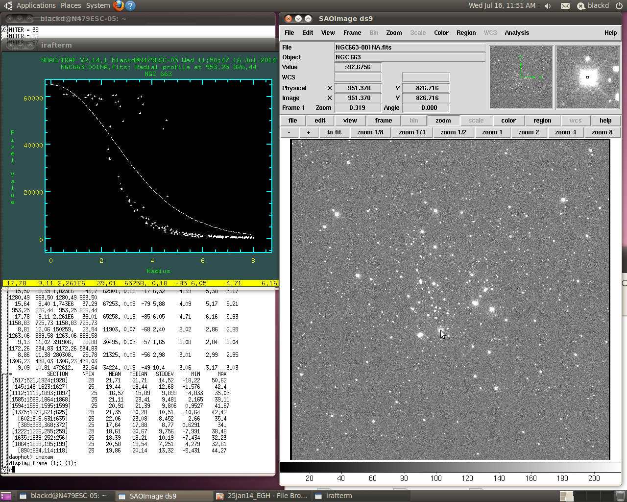
Light curve for a saturated star – the top of the curve is a plateau. The High Good Datum is just below the plateau.

Third, you hover over ten stars again and press the “R” key. This will pop up a graph showing a light curve for that star. Two numbers must be written down: the High Good Datum Point and the PSF radius. The HGD is the height of the curve on the vertical axis, in photon counts, and is usually in the 20-60,000 range. If the star is saturated, the curve will appear flattened and spread out on top, so the HGD is the last point vertically that is providing good data. The PSF radius is the horizontal axis where the light curve flattens out to the background. It’s all a signal-to-noise problem: how far out do you look for stray photons from the star? As far as you can still see them without blending into the basic background noise.

These four values can be used to determine remaining parameters, such as the fitting radius (about 1.4 times the FWHM) and the threshold sharpness (about four times sigma). The header of the .fits file should contain two other values required: the read noise and gain, which is read from the CCD sensor itself.

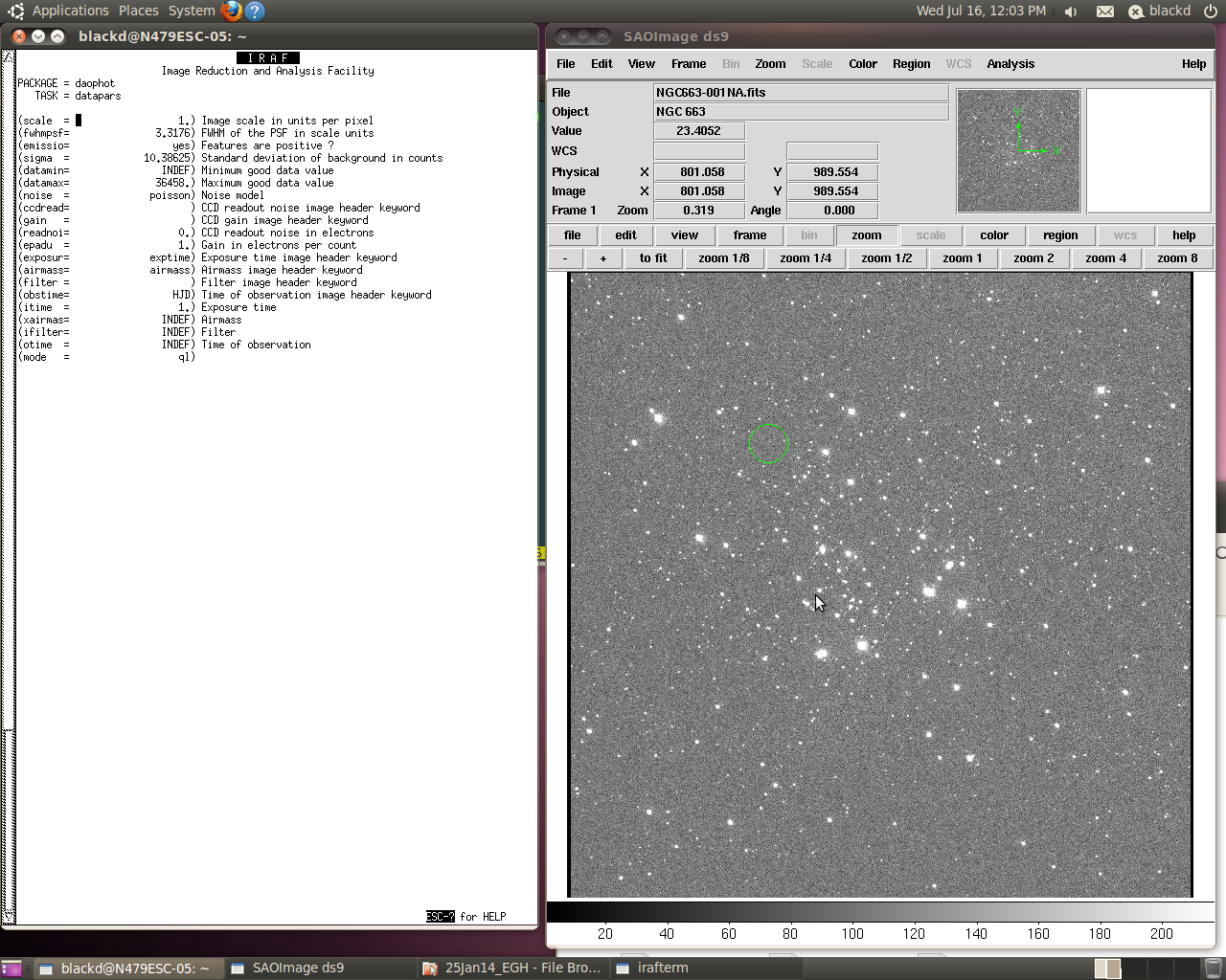
Setting the parameters for the Datapars function using the EPAR command.

Step 2: Setting Parameters

Once you have determined the correct parameter settings from your .fits image file, the next step is to set them in DAOphot. In IRAF, to set parameters one must use the “epar” command (for “edit parameters”). Then you type in a series of commands such as “fitskypars” or “datapars.” You use the arrow keys to scroll down and type in the new numbers. To get out of one screen back to the daophot prompt, you type in “:wq”.

Step 3: Running DAOphot

Once the parameters are entered, you will run through a series of steps to set up and run the photometry analysis using the point spread function, which you must do in the correct order. These include the following:

Coordinate file created by the DAOfind command. This one is for NGC752, which is older and sparser than NGC663 or 659.

A – DAOFind: This command asks you to enter the .fits file to analyze, then walks through the parameters (you can set them here individually as well) and ends by creating a file with the coordinates of every star detected in the image. Depending on the threshold setting, you can get hundreds of stars in a densely packed open cluster. It saves automatically as a .coo file. If you are doing more than one frame for that night, you will want to use just this one original coordinates file for all the frames, but checking to make sure the stars stay lined up. It is also a good idea to load the .coo file into the DS9 frame to make sure the stars are selected properly. They will have small green circles around them. You must use the “Region-load” tabs and navigate to your file, selecting the “all files” option and loading it in as an “xy” and “physical” file.

B – Phot: This command loads the .coo file you just saved and does the initial uncorrected photometry. It asks you to load the appropriate .fits file, walks through the parameters again, and outputs a .mag (magnitude) file.

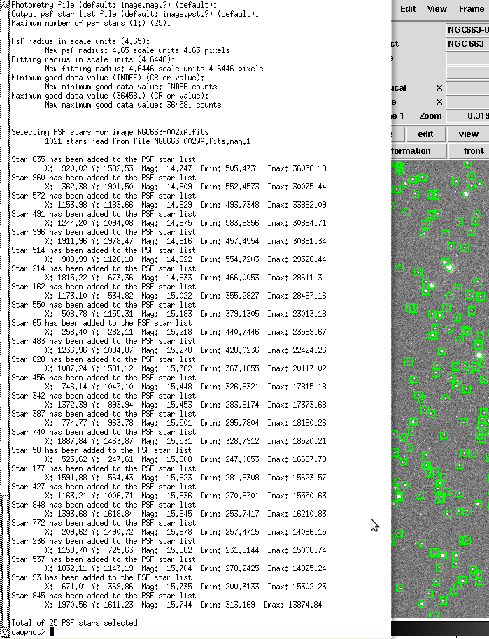
The PSTselect function, which selects a sampling of 25 stars to determine the point spread function.

C – PSTselect: This command selects 25 stars (by default) as representative of the image to determine the profile for the point spread function. It loads the .fits file, uses the .coo and .mag files already saved, and outputs a list of 25 stars as a .pst file. If you have it set to Automatic, it will just list the stars. If you set it to Interactive, a 3-D Gaussian curve of each star pops up and allows you to accept or reject the star. If it has a humpback or shoulder, it is overlapping another star and should be rejected. But it had issues when I tried Interactive mode – it kept giving error messages later on – so we decided to simply accept the automatic setting.

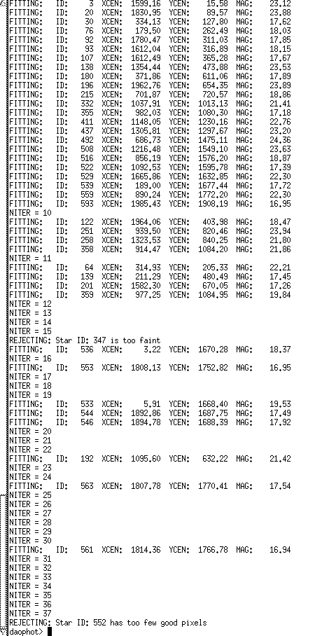
D – PSF: This command does the actual point spread function. Using the previous files, it takes the 25 sampled stars and applies the same algorithm to all of the stars in the .coo file. We had the type of PSF algorithm set to automatic, so it ran through the parameters, then used several analysis functions such as Moffat25 or Penny2, then picked the one with the best fit and output a .psf file. It takes a bit longer to output these curve fits, so wait for it! It also does several passes through the data. As it does, it reconstructs the curves of saturated or overlapping stars.

E – Group: This command groups the data from the previous step’s passes and prepares it for the final corrected photometry. It outputs a .psg file.

The final data table of star numbers, positions (x and y), corrected magnitudes, and errors in the ALLSTAR function. This saves a .als file that can be imported into a spreadsheet.

F – Allstar: This is used if you’re working with large numbers of stars (as I am) whereas Nstar is used for smaller samples. Again you load in the .fits file, walk through the parameters, and after the HGM is returned, it spits out a lot of data, with star number, position (x and y in the .fits image), magnitude, error, etc. It saves it as an .als file. This is the data you will use for analysis. It also ouputs an .arj file, which are the rejects, stars that were too dim or too close to the edges to analyze. The function integrates the volume under the corrected star curves for each star, counts all the photons inside, and compares them to get a list of apparent magnitudes.

Whew! What a process. I went off of the DAOphot manual and student notes, including a notebook left in the computer lab as a reference by the TAs who help students work through this process for the Physics 329 class. But the person who wrote the notebook has very small, densely packed handwriting. Other notes are sparse, more a list of steps without explanation. It took me several days to work through this the first time, using data that had been acquired back in January, 2012, for M67. I decided to start here because it is a well-studied cluster, and quite old, so it should show a variety of stellar processes going on. I felt quite a sense of accomplishment to finally get it to work and spit out the .als file. I did four frames altogether – two with a narrow band Hydrogen alpha filer and two with a wide band Hydrogen alpha filter. It was Friday afternoon when I finished. After three weeks, I finally had data to work with.

Now I have to get that data into a spreadsheet, clean it up, and start my analyses. I have 714 stars to work with, so it will be a large spreadsheet. I’ve also decided to prepare a proper manual with screen captures that a novice high school student could use to successfully navigate DAOphot. I don’t want anyone else to have to learn it from scratch!