Version 2

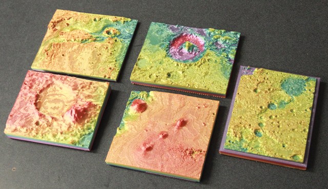
3D printouts of sections of Mars using the Mars MOLA terrain data from NASA’s Planetary Data System Geosciences Node. The sections are, from upper left clockwise: Kasei Valles, Gale Crater, north of Argyre Planitia with Holden Crater, Mons Olympus and Tharsis Plateau, and Jezero Crater.

As a teacher or Mars enthusiast, have you ever wanted to 3D print custom Mars terrains? For example, as the Mars 2020 Perseverance rover prepares to land in Jezero Crater on Feb. 18, 2021, would you like to print out a 3D model of the crater or other places on Mars? This post will teach you how to do just that using a recent version of Adobe Photoshop, an online 3D program called SculptGL, and your favorite slicing and 3D printing software/hardware.

I have written previously about using Mars MOLA altitude data in your science classroom. To get the highest resolution .img files of Mars into a usable format for printing, I recommended using a small utility program from the National Institutes of Health called ImageJ, which allows you to open the .img files and resave them in various formats if you know the exact pixel dimensions and bit depth of the data. I have created a video of the first version of this process using ImageJ on my YouTube channel created three years ago; it can be found at: https://youtu.be/kzdO9PANu_8.

The NASA webpage for the Mars MOLA data. It is part of the Planetary Data System (PDS) Geosciences Node at the Washington University in St. Louis. You want to select the Mission Experimental Gridded Data Records (MEGDRs) link.

I have recently purchased a new Mac computer running MacOS 10.15 Catalina, and have not found a way to get ImageJ to work on this machine (if you know how, please let me know). I have purchased updated Adobe software including the newest version of Photoshop and have experimented with methods for getting the MOLA data into a 3D model using Photoshop’s new 3D features. It cannot read the .img MOLA data files directly, so I have had to use another source. The results have been good, although I have usually had to run the models through another program to flatten the vertical exaggeration and provide a supporting base before I can successfully print them on my 3D printer.

The high resolution MOLA data grid, at 128 pixels per degree or about 1 pixel every 30 meters. For 3D printing, you will want to use the Topography data. Each quadrant is named by the latitude and longitude of its upper left corner. The grid itself shows the coordinates of the upper left and lower right corners. You will need to look at the .lbl metadata file to see the exact number of data points for rows and columns and the bit depth (16 signed) for each pixel in order to open it in ImageJ.

This post will work you through the steps, including where to find the data, how to turn it into a 3D model, and how to prepare it for printing. The end results, when printed with color-changing PLA filament, have been quite successful.

Step 1: Finding the Data:

The high resolution MOLA data is located at the Planetary Data System Geosciences node at the Washington University of St. Louis (WUSTL) at this website: https://pds-geosciences.wustl.edu/missions/mgs/mola.html. You will need to click on the Mars Experiment Gridded Data Record (MEGDRs) link to get to the actual data, then scroll down to the bottom of the page to find the highest resolution data set, which is 128 pixels per degree on Mars, or about one pixel every 30 meters. The best data for 3D printing will be the topographic data, or files beginning with “megt.” The numbers after give the the latitude and longitude of the upper left corner of the section, so you will need a map of Mars to know what area you want to download. For the MOLA data, Mars has been divided up into a a 4 x 4 grid with 16 sections. Clicking on the megt-.img file you want will start the download process. These files are fairly large, so it will take a few minutes.

If you are having trouble getting ImageJ to work for you, a less detailed grayscale image of all of Mars is available here: https://astrogeology.usgs.gov/search/details/Mars/GlobalSurveyor/MOLA/Mars_MGS_MOLA_DEM_mosaic_global_463m/cub

Web page for the lower resolution full Mars data. If used in Adobe Photoshop, the file will have a bi-gradient problem due to elevations lower than martian “sea level” having a negative value. This problem is easily fixed.

This map has a resolution of 463 meters per pixel but is still good for 3D printing. The colored prints of Jezero Crater, Tharsis Palteau, Gale Crater, Kasei Valles, and north of Argyre Planitia came from this image and had to be reduced in size even more before printing. The file is a 2 GB .tif, and if loaded into Adobe Photoshop will show a bi-gradient problem that I will discuss how to fix below.

Step 2: Loading and Converting the Data:

To use the data in ImageJ, you will need to look at the megadata file, or .lbl file. It will tell you that each grid has 5632 rows and 23040 columns and that the data is 16-bits per pixel and signed, meaning that there is an arbitrary “sea level” in the data with positive and negative values above or below that line. Once the .img file is downloaded, it can be loaded into ImageJ using File-Import-Raw. Choose the file you have downloaded, and it will then ask you for the columns (23040 in the newer data, 11520 in older versions) and rows (5632). Choose “16-bit Signed” from the Image Type pulldown menu, 0 for the offset, 1 for number of images, and 0 for the gap. Leave all the checkboxes at the bottom unchecked and click OK. Your section of Mars will then load and show as a grayscale heightmap. You can then save the file as a PNG.

Menus in Adobe Photoshop for converting a grayscale image (such as the MOLA data) into a 3D model. Choose “Solid Extrusion” from the final menu.

Step 3: Creating a 3D Model:

Using MOLA data through Image J: The file will be too large for most 3D printers and software to handle, so I recommend cropping it inside Adobe Photoshop. Before Photoshop had 3D tools, I previously used a program called Daz3D Bryce to load in the cropped image and create the 3D model. I could apply an altitude sensitive gradient texture to the model and render out images and animations, such as the one shown here of the nothern Argyre river channels through Holden Crater. However, Photoshop can now create 3D models directly.

A 3D render of MOLA data showing the area north of Argyre Planitia, with Nirgal Vallis and Holden Crater.

To do this, load in the entire section image and crop it to the desired area. You may want to experiment with the resolution of the final image depending on how much data your 3D printer can handle. I had to reduce it somewhat. I then choose the 3D menu, then “New Mesh from Layer,” then “Depth Map to . . .” and choose “Solid Extrusion.” The grayscale image will be converted into a 3D model that can be saved as a WavefrontOBJ. This model will have its vertical scale exaggerated, so you will need to reduce its height, which I do in a free online browser-based program called SculptGL (see below).

This is the grayscale image of Gale Crater converted into a 3D model in Adobe Photoshop. It’s height is exaggerated and will need to be reduced in SculptGL.

Using the Lower Resolution Image: If you are using the lower resolution image of Mars and not ImageJ, you will need to solve the bi-gradient problem before converting it into a 3D model. To do this, load the entire Mars .tif file and crop it to the area you wish to print. You will see that the low-lying areas of Mars have a light gradient and the high altitude areas have a dark gradient and the edge between them is the arbitrary sea level of Mars. This is caused by the fact that the original data has negative altitude numbers, which Photoshop cannot handle (what is a negative gray, anyway?) so it converts the negative numbers into positive numbers.

To solve this, use the Magic Wand tool, making sure to uncheck the anti-aliasing checkbox and to set the tolerance to about 50 and to turn off contiguous. Then click on the lighter gradient area. The entire light gradient should be selected. You can save this selection if you want, but should not need to.

To solve the bi-gradient problem, you will need to use the magic wand set to a tolerance of 50 and with anti-aliasing and contiguous turned off to select the light areas. Then choose Adjustments-Levels and set the white output slider to 128 and the dark input slide to the edge of the curve to stretch out the light gradient.

Go into the Image-Adjustments-Levels window and move the white Output Levels slider to 128. Then take the dark slider in the Input Levels area and move it over to the edge of the light curve, somewhere around 240. Keep the midtones slider at 1.00 and the white slider at 255. You will now see the light gradient areas (low-lying sections of the model) turn into a dark gradient.

Now invert your selection, which should now select all of the dark gradient high-altitude areas. Go into the Image-Adjustments-Levels window again and move the black Output Levels slider to 128 and the white Input Levels slider to the edge of the light curve, which could be somewhere between 12 and 80. Keep the midtones slider at 1.00 and the black slider at 0. You do not want the highest elevation areas to “bloom” white or you will get a plateau, so it may take some adjustment to get the best range of colors. The dark gradient high areas will now become a light gradient. If you use the eyedropper tool and click on a pixel next to the sea level (right by your selection marching ants) and go into the color picker, you will see that the pixels on both sides register an RGB color of (149, 149, 149) or so. This procedure should eliminate any strange ridge effect at the boundary between the gradients.

Here are the settings for fixing the dark (high altitude) gradient area. Inverse your selection from the first fix, then choose Adjustments-Levels again and set the dark output slider to 128 and move the white input slider over to the edge of the curve as shown. You can then deselect and save. The heightmap is now ready to turn into a 3D model as shown above.

You can now deselect, change the resolution if needed, and convert the corrected image into a 3D model as outlined above.

Step 4: Reducing the Vertical Exaggeration and Adding a Base:

SculptGL is a free browser-based program similar to Sculptris. It can be used to model a sphere or other object as a virtual ball of clay, with very impressive features. Check out some YouTube tutorials and play around with this program; you will love it! It can also modify existing .STL or .OBJ files.

Gale Crater obj model in SculptGL. It needs to have its height flattened using the Transform tool.

To flatten the Mars model, choose “Scene” and delete the scene to get rid of the ball of clay. You can then load in your Mars .OBJ file. On the right side of your screen is a pulldown menu listed as “Tools.” Choose “Transform” at the very bottom of this menu. A transforming tool will appear next to your model. Choose the blue box, which will change the size of the Z axis (depending on the orientation of your model) and push the box in so that the height of the model will be more realistic. Be careful not to rotate the model. You will probably want to save your model at this point under Files – Save .OBJ or Save .STL depending on your preference. This will save a higher resolution version of the model.

Gale Crater model in SculptGL after flattening and remeshing. Choose the Topology pulldown menu, change the resolution to about 250, then click on the Remesh button. This will reduce the resolution of the model and make it printable. You will then need to build a base on it by adding a cube, merging the models, and exporting as an .STL or .OBJ for printing.

Depending on your printer’s capacity, you may need to reduce the resolution of this model by going to the Topography tab on the right side, then move the Resolution slider above “Relax topology” to the right to around 250 (higher if your 3D printer and slicer can handle it) and click on the Remesh button. The model will become less detailed but won’t choke your printer.

3D print of Gale Crater using a color changing filament. My layer height was .27; a smoother model with less terracing can be achieved with thinner print layers.

It may be, depending on the range of your gradients in the original image, that your deepest areas cut all the way to the bottom of your model. If so, you may want to add a base plate to your model to prevent it breaking in two when you remove it from your printer’s build plate. To do this, choose Scene-Add Cube and use the transform tool to shrink and move the cube so that it is just barely touching the bottom of your Mars model. Your deepest crater should show a pixel of peach color in its deepest recesses. Hold down shift and select both models, then choose Scene-Merge Selections to create one final model. Export it and you are now ready to slice and print it.

Step 5: Printing the Mars Terrain:

These steps depend on your slicing software and 3D printer. Supports will not be needed. As a suggestion, try using some rapid color-changing PLA filament. This will give you the appearance of a topographical map; I used a silky textured rapid color-changing filament successfully to create the models shown here. I had my layers set to .27 mm; if you choose smaller layer thickness, you will get a smoother model but longer print times.

3D print of Kasei Valles on Mars. The color changing filament provides a nice topographic map effect. You can see the terracing because my layers are .27 mm thick. You can get smoother results with thinner layers, but some terracing will always be there unless you tip the model at 45 degrees.

An option to try if you want better smoothness in your elevations is to use 3D software to tip the model at a 45 degree angle, build a frame around it, and create supports. You will get less of a topographic levels effect this way, but you will not be able to use color-changing filament to as nice of an effect. In the model shown here, the resolution of the Kasei Valles model was low but the stand and frame worked well.

One final point to consider is that 3D printers will tend to trap in on negative areas, such as craters and river channels or the canyons of Noctis Labyrinthis in the printout of the Tharsis Plateau, so that they become thinner than they should be. This is a common problem with any kind of printer, 2D or 3D, and why you need to make letters thicker than you expect when printing reversed white letters on a dark background. I do not know how to fix this in my 3D prints without making the models inaccurate. Let me know if you come up with a solution.

You can use this process for the Lunar LOLA data, also stored at the PDS Geosciences node to make models of the moon, which we will be using for our ExMASS program participation this fall. For Earth features, I use the USGS EarthExplorer website to download features such as this image of the Book Cliffs in Utah and 3D print them using this same procedure. I printed out a section of the Grand Canyon with the Kaibab Plateau that forms the North Rim in purple and the bottom of the inner gorge in yellow using the color change filament.

3D print of Jezero Crater on Mars, where Perseverance will land in February 2021. The river inlet in the upper left area of the crater is hard to see because of the trapping problem mentioned – thin channels tend to become closed off and thinner than they should be since the filament tends to expand slightly as it prints. The delta deposits next to the landing ellipse are just visible at the mouth of the inlet channel.

I created a Powerpoint of this process which I presented at the virtual 2020 International Science and Engineering Fair and at a virtual training session for teachers for the Greater New Orleans Science and Engineering Fair. It may be useful for you in preparing your students for 3D printing of Mars, moon, Mercury, and Earth terrains. I hope you enjoy the process and get some good results. Feel free to experiment and, as always, let me know how it goes.

Here is a .pdf of this process that was saved from the Powerpoint I created for the ISEF and GNOSEF presentation:

Using 3D terrain models-GNOSEF-s