My version of the Drake Equation, which uses the total number of stars in our galaxy instead of the rate of star formation. Many of these variables have been narrowed down using advanced space telescopes, but the final term, the lifetime of a civilization, winds up being the critical factor.
by David Black
It has been two years since Lily wrote the article in my previous post and I am only now putting together the 4th edition of our Ad Astra Per Educare student newsletter which will include her article. At the time that Frank Drake created the equation in 1961, hardly anything could be answered about any of the variables in the equation except perhaps the first variable about the rate of star formation per year in the Milky Way galaxy, which at the time was estimated to be about three stars per year. With additional data and the advent of space telescopes, we are beginning to get ever better estimates of some of the variables.
One thing that has always puzzled me about Drake’s equation is the inclusion of this first term. Since it is a yearly estimate, the final answer must be the number of communicating civilizations that come into existence per year, which seems an odd way of looking at it. We want to know the total civilizations out there that we might converse with, not just the newbies like us. Carl Sagan spoke of how, given how many of these factors were considered to be close to 1 (or 100%) if given enough time, the truly limiting factor is the final one, the life-span of a civilization where they are able and willing to communicate over interstellar distances. This is why he was so adamant about preserving the Earth and getting rid of nuclear weapons. He wanted us to last long enough to become part of some great Encyclopedia Galactica, a galactic storehouse of the wisdom of all civilizations.
If we do want to estimate the total communicating civilizations, I suggest a modification of the Drake Equation. Here is my own version of it:
N = Stot • fm • fFGK • fp • f HZ • fl • fi • fc • L
N = the total number of communicating civilizations at any one time.
Stot = the total number of stars in our galaxy, which is around 200 billion based on mass estimates.
fm = the fraction of those stars that have high metallicity, such as our sun. These are primarily Population I stars compared with the metal poor, older Population II stars. For life to exist, the proper elements including metals must be present, and the older metal-poor stars are poor candidates. That gets rid of about half the stars, as fm is about 0.5.
fFGK = the fraction of those stars that are like our sun, with long enough life spans for intelligence life to evolve and stable enough to not have UV flares or small habitable zones like red dwarf stars. Counting the number of such stars in the space around us out to 15 light years (this is where we pulled out our 3D model), we see there is one F type star, three G stars, and five K stars out of about 45 nearby stars, or 9/45 or 0.2.
fp = the fraction of those stars that actually have planets, which we know is near 100%, probably about 0.9 to be conservative, based on all the planets we are currently finding.
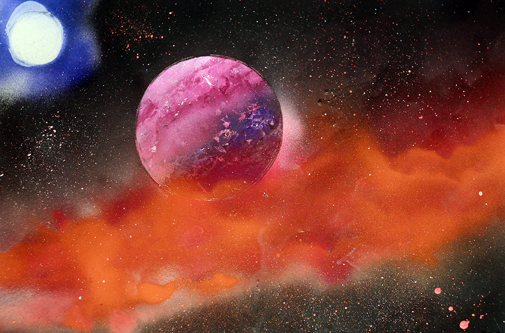
My astrophysics students created these exoplanet paintings using spray paint and various circular masks like bowls and platters. This shows an orange dwarf star with a purple exoplanet orbiting.
fHZ = the fraction of those planets found inside the habitable zone (HZ) of that star. Based on various planetary systems we have detected, if appears this number is about one in four or 0.25.
fl = the faction of those planets that actually evolved life on them. This becomes hard to estimate since we only have one example of life evolving so far. However, we do know that as soon as conditions settled down after the Late Heavy Bombardment ended, life evolved rather quickly within a hundred million years or so. So this number also approaches 1, given enough time. To be conservative, let’s say it is about 0.8.
fi = the fraction of planets with life that evolve intelligent life. This is where I disagree with Drake’s initial estimate that if life hangs on long enough, it will eventually evolve into intelligence. There is no proof of that and it took a rather lengthy time to happen on Earth, despite several near misses. Certainly there was impetus for intelligence during the Mesozoic, what with large predators running amok, but the rodent-like creatures were too small (a necessity to avoid the large predators) and intelligence never happened. So there have been intelligent creatures capable of using tools for the last three million out of 3.8 billion years since life first evolved. This gives us a limiting factor of about 3/3800 or 0.00079.
fc = is that fraction of intelligent creatures that develop technology capable of sending messages over interstellar distances, which for us occurred in 1932 with the first television broadcast capable of reaching beyond the ionosphere. It was sent from the opening ceremonies of the summer olympics, were held in Berlin that year, and hosted as master of ceremonies by none other than Adolf Hitler himself, with a parade of goosestepping Nazis. Yes, Hitler is our ambassador to the stars and there is nothing we can do about it. That gives us 90 years that we’ve had the technology to send signals, or 90 out of 3 million years, a factor of 0.00003.
L = the number of years a civilization will be capable of sending out or detecting signals. If it is only a hundred years or so for us, if we destroy ourselves sometimes soon, then the numbers look grim. But if we can overcome our adolescent tendencies for self-destruction then we might keep radio technology around for a long time, perhaps 10,000 years. This is the real kicker – it all depends on surviving long enough to become a part of the intragalactic conversation.
As a project in my STEAM class this summer my students learned pyrography, or wood burning. I created this little saying (Bonus points if you know its origin) as a demonstration.
Putting all these numbers together, we get:
200,000,000,000 • 0.5 • 0.2 • 0.25 • 0.9 • 0.8 • 0.00079 • 0.00003 • 100 and we get: 8532 communicating civilizations in our galaxy. That’s still a decent sized number. Tweak the numbers such as adding to the lifetime of a civilization and there could be more. Other estimates put the number at less than 1.0, which would mean we are an oddity and possibly alone in the galaxy.
Enrico Fermi was famous for asking a question that is now known as the Fermi Paradox: If there are so many civilizations out there, why haven’t we heard from them by now? Why the great silence?
If you take 8532 worlds and spread them out randomly throughout the spiral arms of the Milky Way (where the metal-rich stars are found), which is 100,000 light years in diameter and is basically disk-shaped, you can use the formula for the volume of a cylinder with a radius of 50,000 light years and a thickness (height) of about 1000 light years. This gives an overall volume of about 7.85 trillion cubic light years. In all that space, 8532 civilizations will be greatly spread out, probably thousands of light years apart. The answer to Fermi’s Paradox becomes obvious: we haven’t heard from anyone because our little Nazi parade has only been traveling for 90 years. No one has heard us yet, if our signal is even strong enough to be picked up. Maybe that’s a good thing.
There have been proposals to send out other, stronger signals and to send them in a tight beam to probable star systems instead of broadcasting in all directions. We’ve sent plaques out on the first space probes to go beyond the solar system, the Pioneer 10 and 11 and Voyager 1 and 2 probes. But it will take tens of thousands of years for them to reach even the closest star systems. We may have to wait awhile before we join the conversation.
I have now completed the fourth edition of Ad Astra Per Educare and it can be downloaded here:
A spray painted exoplanet scene created by my astrophysics students, summer 2022
Written by Lily M.
In 1961 an astronomer named Frank Drake created the Drake Equation. He created it for a way to understand the factors involved in finding life outside our Earth in our galaxy and to roughly calculate the amount of life that can communicate with us. The equation he developed is the following:
N = R* • fp • ne • fl • fi • fc • L
It is a complicated equation and contains quite a few variables.
N means the number of extraterrestrial civilizations we as humans can communicate with.
R* is the rate of star information, which we now know to be about 1.5 stars per year.
fp is the number of stars that have planets. When our Sun was born our solar system organized as a natural consequence with planets forming inside eddies of the solar accretion disk. Astronomers feel that this process would occur around other stars as they formed, and that on average every star should have at least one planet, so this factor approaches 1 or 100%.
A painting of the Epsilon Indi system. An orange dwarf star is orbited by two brown dwarfs which revolve around each other
ne means the number of planets per stars that could possibly support life, or be like Earth. ne is even more difficult to figure out then R* and fp,but was assumed by Drake to be around 3, since there are three planets in our solar system that are or were within the habitable zone.
fl is the fraction of planets that support life and can develop it. With the different types of extremophiles we have found on Earth it looks like life could exists in very hostile environments. This means that fl approaches 1 or 100% with enough time.
fi is the fraction of life-bearing planets that have intelligent life on them, finding out the value of fi is really hard since we only have one example: humans. Some anthropologists still argue on why one of the branches of the ape family evolved into the human species. We don’t really know if this is really unavoidable or just a coincidence. Scientist think that there are other species that could potentially evolve into intelligent beings such as dolphins and chimpanzees. Scientist think that if life could evolve then intelligent life could too, given enough time, since it has happened on Earth and there is no reason to think Earth is a special case.
fc is that fraction of planets with intelligent life where that life is willing and able to communicate with us across interstellar space. Scientist believe that if there is intelligent life out in our galaxy that they will eventually advance to a technology level to send out a signal into space. Knowing the human species, we can only guess that if there is another human-level species they would have either deliberately or accidentally shown that they exist by now. Which could mean that fc could be as high as 1.
A system of exoplanets with two gas giants and a habitable moon
Finally, the last letter L means the time span that the other life can communicate with us. The Earth’s population has grown so much over the past few centuries that the human species has the potential to destroy itself with man-made catastrophes, wildlife disasters, diseases, and nuclear war. If we all start to have a pessimistic view on this then we cannot be sure that human race will live through to the next century, that we will destroy ourselves and our advancement in technology will only have existed for a couple of centuries. It is difficult to say if another species will have the same rate of technological advancement or will have the same tendencies for self-destruction. Scientist think that L is approximately 200 to 10,000 years.
Putting in all the estimates for these variables we come up that N would be about 50, or 50 communicating civilizations per year would arise in our galaxy. The Drake Equation does not have a concrete solution yet because the last four variables are very hard to figure out. You may also have heard of the Drake Equation as the Green Bank equation or Green Bank formula, as the first meeting of astronomers interested in SETI, or the Search for Extra-terrestrial Intelligence, occurred at the Green Bank radio telescope facility in West Virginia. Carl Sagan was one of the astronomers at that meeting, and brought up the Drake Equation in his television series Cosmos. The Drake Equation has been a very popular equation to help us identify the factors we need to solve to look for intelligent life in our galaxy.
An orange dwarf star orbited by a blue gas giant with two red moons
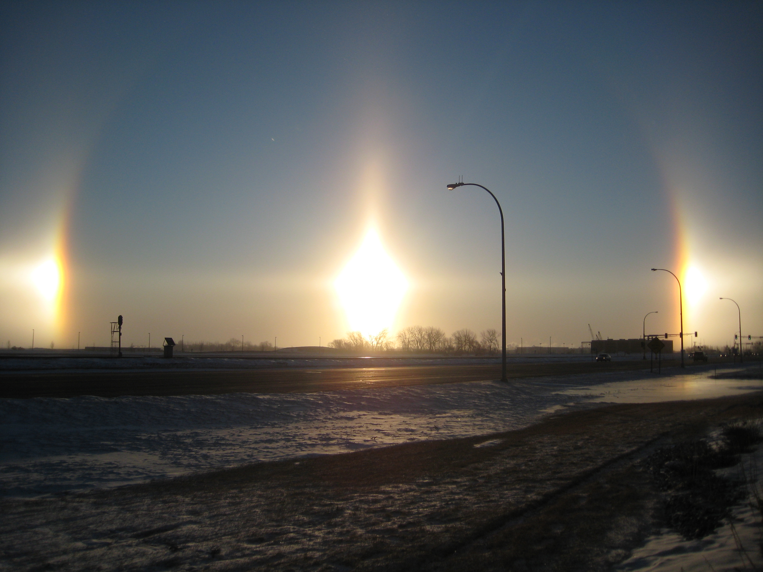
A complex display of halos, sun dogs, and partial parahelic arcs.
It was just past sunset on a cold, clear winter evening in early December. I was driving south down I-15 past the small town of Mona, Utah and the small reservoir nearby. I was teaching at a residential treatment center in Provo, Utah but living in a small town 40 miles south called Nephi, and this was my normal evening commute. I wasn’t really thinking about anything, just listening to music, when I saw it: a glowing object to the right and above my pickup truck, following me. It didn’t have any definite edges, and I couldn’t tell how large it was but it appeared to be keeping pace with my truck. The hackles rose on the back of my neck. For about five seconds I was completely freaked out. I was having a UFO encounter!
Sun dogs near Fargo, North Dakota. These are seen when sunlight is refracted through a thin layer of ice crystals.
Then I realized what it was. It was a sun dog, the frequent explanation given by the air force for many UFO sightings, but literally true in my case. You see, the sun had just set from my position at the bottom of the valley, but it was still shining a few hundred feet above Mona Reservoir. The day was cold, one of the first cold days of the year, but the water in the reservoir was still warm. Water vapor rising above the warm water was hitting a cold air layer a few hundred feet up and crystallizing into tiny ice crystals, which were reflecting the sunlight down into my truck window. It seemed to be following me because it wasn’t really as near my truck as it appeared – it was miles away and the reflection moved with me. Another possibility is that the ice crystals were much higher, part of a thin veil of cirrus clouds and the reflection part of a parahelic arc.
As soon as I moved beyond the reservoir, the sun dog disappeared. Some people report seeing these objects suddenly vanish as if they are moving hundreds of miles per hour when really it is just the ice pocket no longer reflecting the sun. I know a teacher who once saw a UFO, and from her description it was pretty clear what she saw was St. Elmo’s fire, or ball lightning, as it appeared as a ball of light following along a fence line after a thunderstorm.
Image of a sun dog in the Nuremberg Chronicles
There have been many historic accounts of sun dogs; the term itself means an object that dogs (or follows) the sun. The Nuremberg Chronicles, a rare book full of wood cut illustrations, includes an image of a sun dog, and to the plains Indians of North America they were considered omens of bad weather and blizzards to come. There is quite a bit of truth to this, as the cirrus clouds that cause them often do precede a warm front which in the high plains can turn into a blizzard.
Other natural phenomena that are mistaken as UFOs include swamp gas, or pockets of methane with traces of phosphine that can bubble up from methanogens deep in a swamp that decompose organic material. Once the phosphine hits the air, it ignites and causes the methane to burn with a bluish light. These fairy lights are called will o’ the wisps and are thought to be impish spirits leading the unwary to their doom. Of course, following a blue glowing light into a swamp is not a very safe activity. Yet another explanation for UFOs is lenticular clouds. When clear air containing some water vapor is forced to rise up over a conical-shaped mountain it will condense to form a cloud which then is whipped in a circular pattern around the peak, creating a lens-shaped cloud formation that can consist of several layers spinning around the peak. They can look like flying saucers.
Does this mean that all UFO/UAPs are no more than lenticular clouds, St. Elmo’s fire, sun dogs, or swamp gas? Or do the many reports of sightings actually have a kernel of truth to them? What about the recent video footage of Navy and Air Force fighter pilots showing some kind of ill-defined objects tracking along with carrier groups? Like any extraordinary claim, for UFOs to actually be alien spacecraft would require extraordinary proof, as Carl Sagan liked to say. Unidentified flying objects only stay such until they are identified or explained.
Funnel shaped lenticular clouds, stacked in layers, formed from powerful rotational winds around the central peak.
During our astrophysics class at New Haven School this summer, students chose from various famous sightings and investigated them with a critical thinking lens. Does the claim make sense? Is their any indisputable evidence? Did more than one person see it, and were they credible witnesses? Their short essays on their chosen sightings are included in this edition of Ad Astra Per Educare, in which we will explore the possibilities of extra-terrestrial intelligences and our search for them, starting with the Drake Equation and ending with the recent sightings by air force and navy personnel. We will look at various methods for detecting exoplanets, and which ones are the most likely to be Earth-like and in the Goldilocks Zone, or Habitable Zone, of their stars. We’ll also look at an intriguing experiment to detect galaxy-wide civilizations by their waste heat signatures, called the G-Hat project. I will put the main articles of this edition into this blog site over the next few weeks, and upload the final version by next week.
I was contacted last year by a reporter for a news outlet called The 74, meaning the 74 million students who are in school in the United States, regarding how I use my UFO encounter in the classroom. She wanted to capitalize on the rash of press about the navy and air force sightings and congressional investigation, and she had contacted people I know at SETI, who put out the word for any volunteers. I said yes so she called me up and I told her my story. And thought nothing more about it.
Then later in the year I had a parent of one of my students say he had seen an article about me in The Guardian, a British world news magazine that I often read for international perspectives. I thought he must mean a different David Black, because there are quite a few of us around. But no, he said it also mentioned New Haven School. Intrigued, I found the article and it was a reprint of the one done by the reporter for The 74. It seems strange to me that my little UFO incident went international. If you want to read the entire article, here is the link:
I think I’ve pretty much used up my 15 minutes of fame.
A spray-painted image of the Epsilon Indi star system, with the main K-dwarf star in the upper right and the two brown dwarfs, which orbit around each other, in the foreground.
As a separate but related assignment, my students created exoplanet paintings similar to the ones shown in our previous editions. I had 12 students in the class, used better equipment, and most students did two paintings, so I have more to choose from. Their paintings provide most of the illustrations in this 4th edition.
I hope you enjoy the readings and student analyses. This is the fourth of seven editions that use articles written by students at New Haven School. Because of the nature of the school, I cannot provide the students’ full names due to privacy concerns. In most cases the students have worked through three drafts of their essays with peer and teacher review. I think they have done a marvelous job. Enjoy!
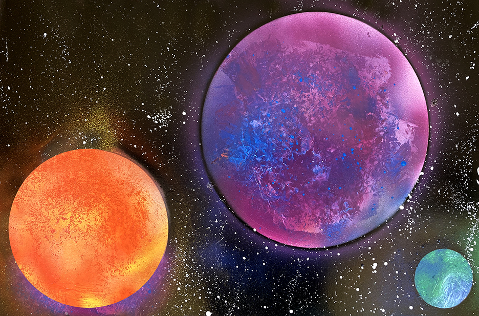
Another spray-painted illustration of a purple planet orbiting an orange giant star.
A Tour of the Star Systems within 13.0 light years of Earth.
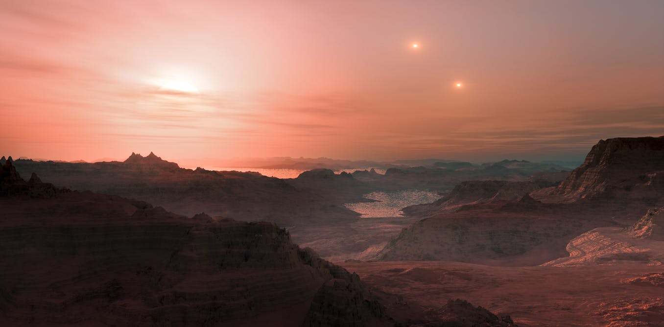
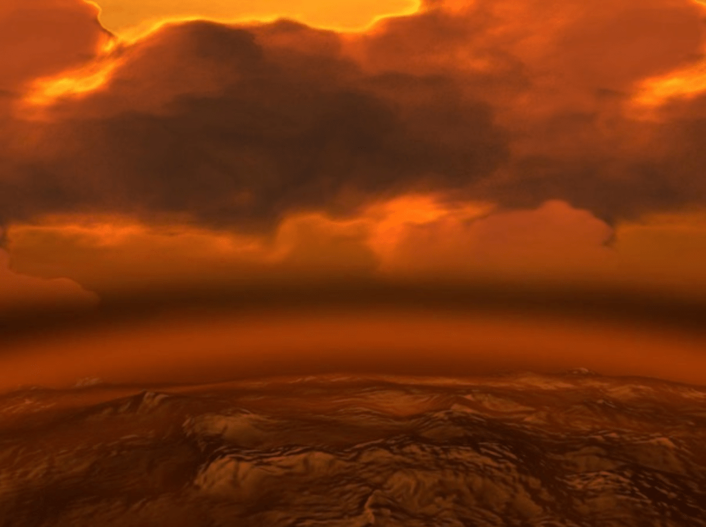
An artist’s rendition of what the surface of Proxima Centauri b might look like.
A map of the nearest stars, from Space.com.
As a media design teacher at Mountainland Applied Technology College from 2000-2009, I created an activity to teach layout design and desktop publishing software with students creating their own version of newsletters. They had to arrange articles I had written about the nearby stars. I used the same articles for many years, but when I dusted them off for our Ad Astra Per Educare magazine 4th edition on the nearby stars, I found that these articles are quite obsolete. Much has changed. It was time to revise the articles.
In my 2020 astrobiology class, my students took on the challenge. Each student chose two star systems to research and report on. For those stars not chosen or written about, I filled in the gaps and also provided additional details on the stars the students wrote about.
It is surprising how much new information has been found about these stars just in the past year since these articles were written. For example, a new candidate exoplanet in the habitable zone around Alpha Centauri A was reported just this last February. Back when I started researching the nearby stars in the early 1990s, this was a somewhat moribund subject without much interest in the astronomy community since no exoplanets had yet been discovered. Now, everyone seems to be getting in on the planet hunting craze and new discoveries are occurring almost weekly.
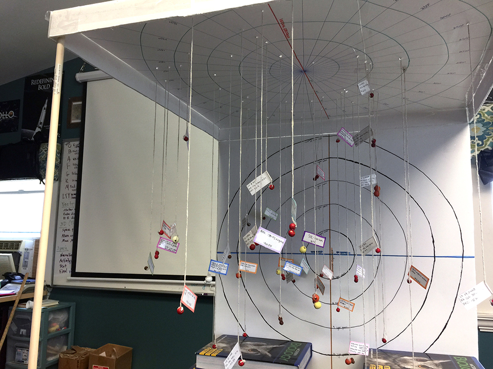
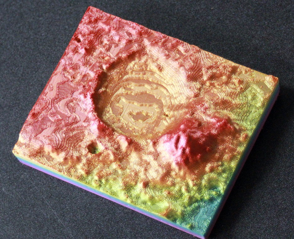
A portable star model made by my 2020 students, described in my previous post.
In addition to describing the star systems themselves, the students wrote sidebar articles on star characteristics such as coordinate systems, classification, naming systems, how we find the distances to them, and other topics. I will post these as our next post.
The Alpha Centauri System: by Hannah T.
The Alpha Centauri triple star system is the closest star system to us, around 4.37 light years away in the far southern constellation of the Centaur. Alpha Centauri A and B are a pair, also known as AB, that orbit close to each other. Proxima Centauri orbits AB and is the closest known star to earth. The declination of Proxima is –62.68, its apparent magnitude is 11.09 and its absolute magnitude is 15.53.
Proxima Centauri is a small red dwarf star of spectral class M5.5V. It is exactly 4.244 light years away and the right ascension is 14h 29m 43s. This star was discovered by Robert T. A. Innes in 1915. Recently in 2016 an exoplanet was located in the habitable zone of Proxima Centauri using the radial velocity method. It is about the size of Earth but would be most likely tidally locked. Because Proxima is a flare star (V465 Centauri), it is unlikely for life to exist there. Proxima now has two confirmed planets, Proxima Cent c is a super-Earth or sub-Neptune planet 7 times more massive than Earth and about 1.49 AU from Proxima. It is therefore too far away to be habitable. There may be a third, sub-Earth sized planet that has not yet been confirmed.
Proxima Centauri is a red dwarf flare star.
Alpha Centauri A, also known as Rigil Kentaurus (“the Foot of the Centaur”) is the largest and brightest star of this triple star system. It is a spectral type G2V and is just larger and slightly brighter than the sun, with an apparent magnitude of .01 and an absolute magnitude of 4.38 (compared with 4.85 for the Sun). This is the third brightest star visible in the night sky and is 4.365 light years away. Alpha Centauri A has a right ascension of 14h 39m 36.5s and a declination of –60.83. The corona of a star is the aura of plasma surrounding it; Alpha Centauri A shows coronal variability because of star spots. A recent Feb. 2021 paper from the Breakthrough Watch Initiative used a direct imaging technique and found evidence for one planet orbiting around Rigel Kentaurus with a distance of about 1.1 astronomical units (AU or the Sun-Earth distance), putting the planet in the middle of the habitable zone. Called Candidate 1, its mass would be slightly larger than Neptune, so it would be a gas giant. It could have habitable moons. The observation was made using only 100 hours of observing time, so further observations are needed to confirm that this is a true planet and not a dust disk or observational artifact.
Alpha Centauri B, sometimes known as Toliman (“the ostrich”), is an orange dwarf star of spectral class K1V with a mass of .907 that of Sol. This star’s apparent magnitude is 1.34, and its absolute magnitude is 5.71. A planet was proposed using radial velocity in 2012 but it has since been refuted as an artifact of data analysis; another candidate planet (Alpha Centauri Bc) was proposed in 2013 using transit data but has yet to be confirmed. It would be slightly smaller than Earth with a 20 day orbit, so not in the habitable zone.
Distances to the nearest star systems compared.
As the closest star system to Earth, Alpha Centauri has figured prominently in science fiction. It was to be the destination of the Robinson family in the Lost in Space series and movie. The character Zephram Cochran, inventor of the warp drive in the Star Trek franchise, lived for a time in the Alpha Centauri system before going missing (“Metamorphosis”). Other episodes throughout the Star Trek universe mention Alpha Centauri. In Babylon 5, an Earth colony is mentioned in the Proxima system and it is the site of a battle between Babylon 5 forces and Earth during the civil war story arc. The planet Polyphemus in the Avatar movie series, orbited by the moon Pandora where the fictional mineral unobtanium is being mined, is located in the Alpha Centauri system. In literature, Alpha Centauri figures prominently in many science fiction novels including The Songs of Distant Earth by Arthur C. Clarke, Foundation and Earth by Isaac Asimov, Footfall by Larry Niven and Jerry Pournelle, Neuromancer by William Gibson, and The Three-Body Problem by Liu CiXin.
Barnard’s Star:
The second closest star system to our sun was discovered by E. E. Barnard in 1916 as part of his proper motion studies. It has the fastest known proper motion of any star, at 10.3 arcseconds per year relative to our sun, making it a very close star. Using parallax with refinements by the Hipparcos and Gaia satellites, its distance has been measured at 5.96 light years. It is a small red dwarf with a mass 0.144 times the mass of our sun and a spectral type of M4.0V. It is located in the constellation Ophiucus at 17h 57m 48.5s right ascension and +04° 41m 36.2s declination. It can only be seen with a powerful telescope and has an apparent magnitude of 9.511.
The nearest single star to the Sun (Barnard’s Star) hosts an exoplanet at least 3.2 times as massive as Earth — a so-called super-Earth. Data from a worldwide array of telescopes, including ESO’s planet-hunting HARPS instrument, have revealed this frozen, dimly lit world. The newly discovered planet is the second-closest known exoplanet to the Earth and orbits the fastest moving star in the night sky. This image shows an artist’s impression of the planet’s surface.
For many years, Peter van de Kamp argued that Barnard’s Star had at least one planet based on his astrometry measurements, which involved measuring the changes in the positions of stars on photographic plates as small as one micron. These arguments were largely refuted in the 1970s when it was shown that the perturbations seen in the plates corresponded to maintenance upgrades of the telescope’s lens. However, in 2018 a candidate super-Earth was announced from the Red Dots project using highly precise measurements of radial velocity with data from the ESO HARPS (High Accuracy Radial velocity Planet Searcher) spectrograph and other instruments over a 20 year period. It is believed to have a minimum of 3.2 Earth masses and to orbit at 0.4 astronomical units and a period of 233 days, putting it beyond the habitable zone. This planet is also disputed, since star spots might produce a similar radial velocity shift. Barnard’s Star is a flare star, as are most red dwarfs, making life on such a planet unlikely.
Based on its slow rotational speed and low metallicity, Barnard’s Star is estimated to be between 7-12 billion years old, making it much older than the sun. A surprisingly large solar flare was detected in 1998, very unusual for such an old star. Smaller ultraviolet and x-ray flares were detected in 2019.
In the Hitchhiker’s Guide to the Galaxy series by Douglas Adams, Barnard’s Star is said to be the location of an interstellar roundabout used by the Vogon Constructor Fleet. It is also a major part of the novels The Garden of Rama by Arthur C. Clarke and Gentry Lee and Hyperion by Dan Simmons.
Luhman 16 A and B: by Navah D.
Luhman 16 is a binary star system with both stars being brown dwarfs orbiting each other at about 3.5 astronomical units (the Earth-Sun distance) and an orbital period of 27 years. The system is actually located in the southern hemisphere in the constellation Vela and is approximately 6.503 light years away from the sun. This very unique star system is also known as WISE 1049-5319 because the stars can only be seen in infrared using data from the WISE telescope. Kevin Luhman, an astronomer with Pennsylvania State University, discovered the stars in 2013. Because they lie close to the galactic plane, where stars are crowded, they eluded discovery until then. They are the nearest known brown dwarfs to the solar system, and the closest system discovered since Barnard’s star in 1916. These stars have not been around for a very long time; they are fairly young for stars at about 600-800 million years old.
A photograph of Luhman 16 A and B, a double brown dwarf system.
For Luhman 16 A, the largest of the pair, is classified as an L8 star with .032 times the mass of our sun and 33.5 times the mass of Jupiter. It has a surface temperature of about 1400 K. Luhman 16 B is a T1 star with a mass of .027 Sols or 28.6 Jupiters. Both stars are located at RA 10h 49m 15.57s and declination of -53° 19m 06s. Luhman 16A is suspected of having a planet, Luhman 16Ab, measured through astrometry with the Hubble Space Telescope in 2013. That planet is now considered unlikely based on further measurements of the system.
WISE 0855-0714:
A sub-brown dwarf of classification Y4 in the constellation of Hydra, this smallest of all stars yet known was discovered by Kevin Luhman using data from the WISE infrared telescope in 2013. It is right at the border between planet and star, and would have only fused deuterium for a short time before starting to cool down. Its surface temperature is 225-260 K, making it about the same temperature as Mars and therefore the coldest known star, but also much too warm for it to be a rogue planet; it must have had an internal heat source suggestive of previous deuterium fusion. Yet it only has a mass of 3-10 times the mass of Jupiter, putting it into the planetary mass range. It is 7.43 light years away and has a high proper motion. There is some evidence from the Magellan Baade Telescope that it may have water clouds. If seen up close, it would have a purple to deep magenta color.
Wolf 359:
This small red dwarf is located exactly on the ecliptic in the southern part of Leo not far from the star Regulus. It is 7.9 light years away and has a classification of M6.5V and an apparent magnitude of 13.54; it can only be seen with a large telescope. It is far too dim to be seen with the unaided eye. Its surface or photosphere has a temperature of only 2800 K, about half the temperature of our sun. At this temperature, chemical compounds such as titanium (II) oxide and even water can exist in gaseous form. It has a stronger magnetic field than our sun due to the complete circulation of materials inside because of convection currents; as a result of this magnetic field, strong X-ray and gamma ray flares can sometimes be observed. It is less than a billion years old and hasn’t had time for these flares to die out as its rotation slows. It is just barely large enough to sustain proton-proton fusion and be considered a red dwarf instead of a brown dwarf, having only 8% of the sun’s mass. Because it is able to convect all of its material, it can sustain fusion for eight trillion years. It is just getting started.
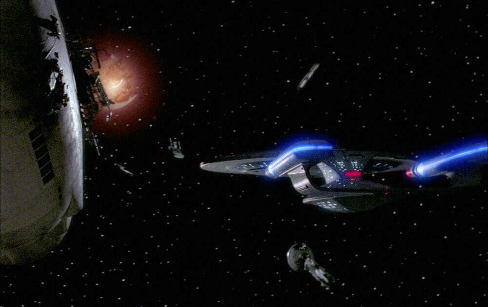
The USS Enterprise D flies through the carnage after the Battle of Wolf 359 in Star Trek: The Next Generation’s “Best of Both Worlds part 2.”
Wolf 359 was the 359th star listed by German astronomer Max Wolf in his 1919 catalog. He was cataloguing stars with high proper motion, knowing they were nearby stars. It is known to have at least two planets. Wolf 350c is a super-Earth with 3.8 Earth masses and near the star, with an orbital period of 2.7 days. It receives three times the energy that Earth does. Wolf 359b (the first to be discovered) is a Neptune-class planet 44 times the mass of Earth with an orbital period of about 3000 days even though it is only about 2 astronomical units from the star. The low mass of the star allows the planet to have such a slow orbit.
Because of its proximity to Earth, Wolf 359 has been the subject of several important science fiction works. Most notably, it was the site for a major battle between Federation forces and a Borg cube on its way to Sector 001 (Earth) to assimilate humanity. 40 starships engaged the Borg, but because Captain Picard had been assimilated, they knew all of his tactical knowledge and easily defeated the Federation. Someone in the Star Trek writers group did their homework and found that Wolf 359 was close to Earth and a likely site for such a battle. However, the Borg are supposed to originate from the Delta Quadrant on the opposite side of the galaxy from our position. Wolf 359 is in Leo, putting it further out from the galactic center than Earth; the Borg would have had to take a very roundabout route to come at Earth from Leo. “Wolf 359” is also the title of an Outer Limits episode where a scientist creates a simulation of Dundee’s Planet in the Wolf 359 system only to see a dangerous life form evolve. In the novel Chindi by Jack McDevitt, a lost spaceship is found in the Wolf 359 system.
Lalande 21185: by Sarah S.
Another red dwarf located in the southern corner of Ursa Major, this star is 8.31 light years from Earth. With an apparent magnitude of 7.5, it is somewhat brighter and hotter than Wolf 359 and may be as old as 10 billion years. It is also known as BD +36 2147, Gliese 411, and HD 95735. It was first listed in 1801 by Joseph-Jerome de Lalande and its proper motion was first measured by Friedrich Wilhelm Argelander for the Bonner Durchmusterung (BD) or Bonn Star Catalog. It has 38% the mass of Sol and a photospheric temperature of 3828 K. Although listed as a flare star, it is rather quiet as far as red dwarfs go.
Friedrich Wilhelm Argelander
Peter van de Kamp claimed in 1951 that Lalande 21185 had a planet based on astrometric measurements using the same photographic plates as for his Barnard’s Star planet claim, but those plates were shown to be flawed. George Gatewood made his own astrometric measurements and claimed that there were multiple planets in the system, although his data remains unconfirmed. Using sensitive radial velocity measurements in the 1980s, Geoff Marcy could not find any planets in the system. However, recent measurements by the HIRES system at Keck Observatory supported there being at least one close in planet with a mass of at least 3.8 Earths and a period of 10 days. Further measurements with the SOPHIE echelle spectrograph showed this planet to have a period of 12.95 days and 2.99 Earth masses, which has been confirmed by other measurements. One other planet orbiting at 2806 days and with 14 Earth masses has also been confirmed, with a third planet suspected between them. Thus, van de Kamp and Gatewood’s claims have been somewhat vindicated even if these are not the planets they claimed to have found.
In fiction Lalande 21185 is the star of the planet Ormazd in Rogue Queen by L. Sprague de Camp (1951) and is one of many nearby stars mentioned by Gregory Benford in Across the Sea of Suns (1983), where it is renamed Ra. In the Revelation Space stories by Alastair Reynolds, the planet Zion orbits Lalande 21185.
Sirius: by Katie T.
Sirius is the brightest star in the sky seen from earth. The name comes from the Greek word meaning glowing/ scorching. Sirius is part of the Canis Majoris constellation, which is also called “The Greater Dog,” and can therefore also be called Alpha Canis Majoris. The star lives up to its name; in ancient Greek times a myth was created. Sirius the star was so hot men would feel weaker, plants would fail to grow, and women would become very aroused. Whenever Sirius first made an appearance, it was known as the “Dog Days” to the Egyptians and signaled the beginning of the inundation of the Nile, the beginning of the their calendar year.
Sirius A (foreground) and B (background) in an artist’s rendition.
A German astronomer, Friedrich Wilhelm Bessel, predicted Sirius B in 1844. The star is part of a binary star system consisting of two stars orbiting each other, with Sirius B as the closest white dwarf to Earth. Bessel made the assumption there was another star, after observing the motion of Sirius A. Following the information provided by Bessel, an astronomer in 1862 discovered Sirius B (the Pup). Alvan Graham Clark was testing the aperture of the largest telescope in America and came across a smaller star orbiting around Sirius A.
You may not think it, but Sirius is even bigger and hotter than our sun. If you observe the sky on a clear day, you may even be able to catch a sighting of the brightest star, using just the naked eye.
In fiction, Sirius Black is the name of the godfather of Harry Potter in the series of books by J. K. Rowling, first introduced in the third book, The Prisoner of Azkaban (although mentioned in the first book as the owner of the motorcycle being used by Hagrid in the first book). He is able to transform into a dog, of course, and he is killed by his cousin, Bellatrix LaStrange, who is also named after a star (meaning “Warrior Woman”). Sirius’ brother is named Regulus Arcturus Black, a double star reference. In Homer’s The Iliad, Achilles is compared with the brilliance of Sirius. Voltaire’s Micromegas describes an alien from a planet orbiting Sirius. In the Foundation series and the novel Pebble in the Sky by Isaac Asimov, Earth is considered to be somewhere in the “Sirius Sector.” Much of the technology mentioned in Douglas Adam’s Hitchhiker’s Guide to the Galaxy series is made by the Sirius Cybernetics Cooperation.
An artist’s rendition of the binary red dwarf system Luyten 726-8 A and B.
Luyten 726-8:
A binary red dwarf system in the constellation Cetus, it is also known as UV Ceti or Gliese 65. They are 8.7 light years away and considered as prototypes of UV flare stars. They were discovered by Willem Jacob Luyten in 1948, have almost equal brightness and orbit each other every 26.5 years. They may be part of the Hyades open star cluster.
Ross 154:
Another small red dwarf single star located in Sagittarius, it was discovered by Frank Elmore Ross in 1925 as part of his lists of new variable stars and stars with high proper motion. It is a UV Ceti type flare star, with a variable star designation of V1216 Sagittarii and average time between ultraviolet flares of about two days. Using highly precise data from the HARPS spectrograph during the Red Dots campaign, Ross 154 is shown to have a rapid rotation of 2.87 days, which corresponds to a young age of less than one billion years. This was the third star, including Proxima Centauri and Barnard’s Star, that was studied in the 2017 Red Dots study. It is of spectral type M3.5Ve and is 9.7 light years distant. It is not known to have any planets, but detecting planets is a challenge because of its rapid rotation and active surface, which produce a great deal of noise in the radial velocity data. In fiction, it is the site of Glory Station in C. J. Cherryh’s Downbelow Station.
Ross 248:
Another unremarkable red dwarf flare star discovered by Frank Ross. It is also known as HH Andromedae or Gliese 905 and is 10.3 light years away, with Right Ascension: 23h 41m 54.7s and Declination: +44.18 °.
Epsilon Eridani:
Also known as Ran (based on a 2015 naming contest by the International Astronomical Union, won by 14-year old James Ott), this is an orange dwarf star slightly smaller and cooler than our sun. It is 10.5 light years away with RA: 3h 32m 55.84s and Dec: -09° 27′ 29.73” and spectral class K2V. It has 82% of the sun’s mass and is a fairly young star, less than one billion years old and perhaps as young as only 200 million years and still gives off appreciable amounts of ultraviolet radiation.
Comparison of the Epsilon Eridani system (top) with the Solar system.
As a close sun-like star, E. Eridani has been intensely studied for planets. This was another star thought to have had planets by Peter van de Kamp but his measurements were later shown to be caused by defective photographic plates. Measurements by the IRAS infrared satellite showed that it still retains at least two dusty rings containing asteroids, one that is about 4 AU from the star and one at about 20 AU. It also has a Kuiper belt analog or cometary cloud about 30 AU out. Clumping in the dust rings was considered evidence that it may have planets, and at least one large exoplanet perhaps 1.2 times the mass of Jupiter is considered to be confirmed now that the Hubble Space Telescope has shown perturbations in the path of Epsilon Eridani using astrometry. This planet has been given the name Ægir by the IAU and orbits the star every 7.4 years at about 3.4 AU, or just outside the inner asteroid belt. Computer simulations of the clumping of dust particles in the rings suggests their may be a second planet in an eccentric resonance orbit. E. Eridani has slightly less metal than our sun, but enough for rocky planets to exist closer to the star.
Because of its nearness and similarity to our sun, E. Eridani was one of the two stars first chosen for listening for alien signals by Project Ozma in 1961 by Frank Drake. No signals were detected. Project Daedalus of the British Interplanetary Society has suggested E. Eridani as one of the possible targets for an interstellar space probe. It has been the subject of many science fiction works, including Babylon 5. In the series, the station orbits at the L5 point of Epsilon Eridani III and its moon. The planet is also the site of the Great Machine that figures prominently in several episodes. In Star Trek, Epsilon Eridani is the system of the planet Axanar, where a famous space battle occurred between the Federation and the Klingon Empire prior to the events of the original series and where Garth of Issus became famous for his battle tactics. It is also mentioned in Space: Above and Beyond, The Orville, and Space Precinct as well as many novels, short stories, and games.
Ross 128: by Julia W.
Ross 128 is a red dwarf star, found in the equatorial zodiac constellation Virgo at RA: 11h 47m 44.4s and Dec: +00° 48′ 16.4”, not far from the star Beta Virginis as seen from Earth. It is a fairly old and quiet star, as red dwarfs go, not exhibiting as many flares a seen in other red dwarfs, although a strong flare was noted in 1972 in the UV band. It is 11.13 light years from Earth with a spectral class of M4V and a mass of 15% that of the sun. It was first cataloged in 1926 by Frank Elmore Ross. It is considered to be an old disk star, and recent measurements by the APOGEE instrument indicate is has nearly the same metallicity as Sol. It does not have the infrared excess that would indicate a dust ring. It is a slow rotator, spinning only once every 165.1 days, because of it old age and the gradual slowing or rotation due to magnetic braking.
Infographic on Ross 128 b.
A great deal of excitement and speculation occurred when an exoplanet, Ross 128 b, was announced orbiting the star in its habitable zone. This planet is slightly larger than Earth at 1.8 Earth masses with about 1.4 times as much energy reaching it than Earth. Although hotter than Earth, its orbit and the quietness of the Ross 128 make this one of the best candidates for life of any exoplanet discovered so far and the second closest habitable zone planet after Proxima b. Ross 128 b orbits every 9.9 days and is close enough to be tidally locked, which, if it has oceans, would make it a candidate as an “eyeball” planet and an Earth-like analog. It is most likely a rocky planet based on its size, orbit, and the parent star’s metallicity.
Radio signals were detected in 2017 by the Aricebo observatory that appeared to be coming from the vicinity of Ross 128, but the Allen Array was able to show that these signals were actually from geosynchronous satellites orbiting the Earth; Ross 128 orbits near the celestial equator near the orbits of many communication satellites.
Gregory Benford, in his 1984 novel Across the Sea of Suns, describes an amphibious alien race living below the ice of a Ganymeda-type exomoon orbiting a planet in the Ross 128 system. They are hiding from extinction caused by a Berserker killing machine called a Watcher orbiting the moon. In the TV series War of the Worlds (2019) Earth is attacked from Ross 128 after picking up a signal.
EZ Aquarii by Lily M.
EZ Aquarii is in the constellation Aquarius and is a triple star system about 11.3 light years away from the Sun and is also known as Luten 789-6 and Glieses 866. Its Right Ascension is 22h 38m 33.4s and its Decl. (deg.) is –15.3. For EZ Aquarii A the stellar type is M5.0V, the other two stars are about the same or slightly smaller. Its magnitude is 12.87. EZ Aquarii may have been found by All of the EZ Aquarii stars A, B, and C are M-typed red dwarf stars and are too faint to be seen by our eyes without help. An interesting fact about EZ Aquarii is that both A and C form a spectroscopic binary that orbit at 3.8 days, with B having an orbit of 823 days. A and B are both flare stars, and the system has no known planets as yet. Its nearest neighbor at this time is Lacaille 9352, which is about 4.1 light years away, making this system rather isolated.
Comparison of Sol (left) with the binary orange dwarf stars 61 Cygni A and B.
61 Cygni
This binary system southeast of Deneb in the summer sky has bright enough stars that they were included in John Flamsteed’s star maps and therefore have a Flamsteed designation from his 1712 Historia Coelestis Britannica. Both stars are old K-type orange dwarf stars (K5V and K7V respectively) and can be seen with the naked eye under clear, dark skies or with binoculars in areas of high light pollution. They orbit each other every 659 years at about 44 AU, having a wide separation. In clear skies, the pair of stars can be resolved with a 10x power pair of binoculars. The proper motion of 61 Cygni was measured in 1804 by Giuseppe Piazzi; this is the only visible eye star system that has a high proper motion and was therefore called “Piazzi’s Flying Star.” In 1834 Friedrich Bessel measured its distance as 10.4 light years using stellar parallax, the first star to ever be measured in this way. Its actual distance is 11.4 light years. There have been claims of a massive planet orbiting one of the two stars which have been controversial. The 2018 data release from the Gaia spacecraft indicates that there are anomalies in the orbits of the stars around each other showing that they are not quite orbiting around their center of mass and that 61 Cygni B is moving too slowly for its mass. This may indicate the presence of an as yet unconfirmed planet around 61 Cygni B. Measurements of the infrared signature of the system show a possible infrared excess suggesting a possible circumstellar dust disc.
Procyon by Cate L.
Procyon A is the brightest star in the constellation of Canis Minor, which means “smaller dog” in Latin, the eighth brightest star in our sky, and is a binary star, which indicates that another star orbits around Procyon. The distance of Procyon A and B from our planet Earth is 11.46 light years away. The right ascension for both stars is 7 h 39 m 18.1 s, and the declination of both stars is 5°13 m 30 s. Their stellar types are F5 IV-V, and DQZ. The first one is yellowish-whiteish and the second one is a white dwarf. The temperature for A is 6,530 K, whereas B is 7,740 K. As a white dwarf, B is the core of a star much like our sun that threw off its outer layers leaving a white hot companion to the slightly cooler and more yellowish A star. The two stars orbit a common center of gravity every 40.84 years in moderately eccentric or elliptical orbits.
Photograph of Procyon (top left), Betelgeuse (orange star top right) and Sirius (middle bottom).
Procyon was known to the ancients and to all cultures, being one of the brightest stars in the sky. In Greek, its name means “before the dog” referring to it rising before Sirius, the dog star. In other non-Greek cultures, it has been known as Nangar, the Carpenter to the Babylonians. The Latin version of Procyon is Antecanis and Arabic names are Al Shira or Elgomaisa and Turkish Rumeysa, the Bleary-Eyed Woman. To the Hawaians, it was Puana, the Blossom and to the Chinese, Nan He San, the Third Star of South River.
The A star is a late main sequence class F star, and will reach the end of hydrogen fusion in its core within the next 10-100 million years, after which it will swell 80-150 times it current diameter and become a red giant.
Procyon B was first proposed by Friedrich Bessel based on astrometric measurements and it was visually confirmed in 1896 by John Martin Schaeberle at Lick Observatory. It was originally a B-type star about 2.59 times the mass of our sun, which came to an end about 1.19 billion years ago after a main sequence lifetime of about 680 million years, making its remnant an old white dwarf.
Struve 2398:
A binary red dwarf system in the constellation of Draco, these stars were first included in the double star catalog of Friedrich Georg Wilhelm von Struve as system 2398. Also known as Gliese 725, the Greek letter sigma is sometimes used to designate Struve catalog stars. Both stars in the system are x-ray flare stars, as are most red dwarfs, and orbit each other with a period of 295 years. They are 11.6 light years away. The B star in the system has two planets, both of about Neptune’s size. One has an orbital period of 91.29 days and the other 192.4 days.
Groombridge 34:
Located in the constellation Andromeda, this pair of binary red dwarf flare stars is ll.618 light years away and was first listed in A Catalogue of Circumpolar Stars by Stephen Groombridge, published posthumously in 1838. They orbit around a common center of gravity in almost circular orbits every 2600 years at about 147 AU. Using radial velocity measurements, two planets have been inferred orbiting around Groombridge 34 A, one a super-earth with 3.03 Earth masses and the other a larger Neptune-class planet with 36 Earth masses.
DX Cancri:
This dim M6.5V red dwarf flare star is in the constellation Cancer and is 11.8 light years away. It is small for a red dwarf, with only 9% of the Sun’s mass and a temperature of 2840 K. It is proposed to be part of a group of stars called the Castor moving group that all had a common origin about 200 million years ago in an open cluster and are moving together as a group while gradually spreading apart. It is not known to have planets.
Comparison of Tau Ceti system (top) with the Solar System.
Tau Ceti by Ruby R.:
This is one of the most important stars near us in that it is a G8V star only slightly smaller and cooler than Sol, with 78% of the sun’s mass. It has a lower percentage of metals than the sun, and is 11.91 light years away in the constellation of Cetus, the whale. It does not have a Greek common name, and was first listed in western catalogs in 1603 by Johann Bayer in his Uranometria. The Calendarium of Al Achsasi al Mouakket of 1650 lists this star as Thalith al Na’amat, the Third Ostrich. It is the Fifth Star of the Square Celestial Granary in Chinese. Estimates of Tau Ceti’s age, based on its metallicity and models of stellar evolution, put it at about one billion years older than our Sun. It is a very stable star, with few if any sunspots and a weak magnetic field.
Because it is the closest single G-type star, it is a Solar analog and has been continually studied for SETI and exoplanet research. It was one of Frank Drake’s original stars for Project Ozma in 1961. Four planets are confirmed to orbit Tau Ceti, designated g, h, e, and f. They are all super-Earths. Planet e orbits every 163 days, putting it at the inner edge of Tau Ceti’s habitable zone with a radiative flux slightly less than Venus, and Planet f orbits at 636 days, putting it at the outer edge with a solar flux comparable to Mars, but with a thick enough atmosphere could sustain liquid water on the surface. Four other planets are suspected to be in the system but are not yet confirmed, although statistical modeling agrees with the detected radial velocities of Planets b, c, and d. With the possibility of 8 or 9 planets, the Tau Ceti system is similar to our own and one of the best candidates to search for life.
Infrared measurements show that Tau Ceti has a thick debris disc similar to our asteroid belt but ten times more dense, and orbiting roughly in the same area as our Kuiper Belt, which would make collisions with any potentially habitable planets more frequent. If there is a large gas giant, as some have proposed (unconfirmed Planet i) then it might have a similar role to Jupiter in deflecting potential impactors. As dense as this dust disc is, it is only 1/20 as dense as the one around Epsilon Eridani. Such dust discs may be common around sun-like stars and may play a role in planet formation; our solar system may be an exceptionally dustless system that had many of its comets and asteroids cleared out early on by a passing star.
In science fiction, Tau Ceti is the system of the planet Aurora in Isaac Asimov’s robot novels as the first settled of the spacer worlds and is the setting of the novel The Robots of Dawn. It is the home world of the roboticist Dr. Han Fastolfe. It is the destination of the torchship Lewis and Clark in Heinlien’s novel Time for the Stars. The planets of Tau Ceti are the setting of Ursula LeGuin’s The Dispossessed. The Downbelow Sation of C. J. Cherryh’s novel of the same name is located on planet Downbelow orbiting Tau Ceti. The Legacy of Heorot by Niven, Pournelle, and Barnes takes place on the planet Avalon (Tau Ceti IV). 100 colonists, sent by sleeper ship, find that ice crystals have built up in their brains while in suspended animation and arrive on Avalon with reduced mental abilities only to be forced to counter the threat of ferocious grendel monsters. In Rama Revealed by Arthur C. Clarke, a group of colonists travel on the Rama II to a node in the Tau Ceti system. In Leviathan Wakes in the Expanse series of novels and TV show by James S. A. Corey, the Mormon generation ship S. S. Nauvoo is traveling to the Tau Ceti system before being commandeered to crash into Eros.
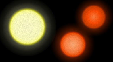
Diagram of the Epsilon Indi system. A double set of brown dwarfs (Ba and Bb) distantly orbit the main K-dwarf star Epsilon Indi A.
Epsilon Indi:
This is an unusual trinary system with an orange K-type dwarf star in the far southern constellation Indus orbited by two T-type brown dwarfs that are orbiting each other and designated Epsilon Indi Ba and Bb. The A star has at least one planet called Epsilon Indi Ab and it has a mass of about 3.25 Jupiters, making it the closest Jovian planet to us. It has an orbital period of 45 years compared to about 12 years for Jupiter, putting this planet much further out. Since Epsilon Indi is an orange dwarf star cooler than the sun, this planet is far outside the habitable zone. The two brown dwarfs are about 1460 AU from the main star or over 37 times the distance between our sun and Pluto (which is 39 AU away from Sol). They orbit each other at about 2.1 AU every 15 years. They have the masses of about 47 and 28 times the mass of Jupiter. The complexity of this system makes it a good candidate for studying the evolution of stellar systems. The size and distance of Epsilon Indi Ab make it a good candidate for direct observation by the James Webb Space Telescope.
Gliese 1061:
Located 11.98 light years from Earth in the constellation Horologium, this small red dwarf was first discovered by Wilhelm Gliese in 1974 when its proper motion was measured, but it was assumed to be much further away at 25 light years. The RECONS satellite was able to measure its parallax much more accurately in 1997 and provide a better estimate of its distance. It is at the lower limit of a red dwarf star at only 11.3% the size of Sol and 0.2% as luminous. Any smaller and it would be a brown dwarf.
In 2019 the Red Dots program announced that the star has three exoplanets: b, c, and d with periods of 3.2, 6.69, and 13.03 days respectively. They are all super-earths with similar masses of 1.38, 1.75, and 1.68 Earth masses. Because of the small size of Gliese 1061, the second planet (Gliese 1061 c) actually orbits just within the inner edge of the star’s habitable zone but would have an equilibrium temperature of 307 °K or 93 °F assuming a similar atmosphere to Earth. It receives 34% more radiative flux than Earth but is so close to its parent star that is likely to be tidally locked with one side constantly facing the star. The third planet, Gliese 1061 d, is also possibly in the habitable zone but on the cool side with 40% less stellar flux than Earth, making it more like Mars. Although its close proximity to the star would indicate tidal locking but it has a fairly eccentric orbit at 0.54, which would tend to destabilize the tidal locking and allow for a day-night cycle. This eccentricity would be a challenge for life.
YZ Ceti:
At 12.11 light years from Earth, this red dwarf flare star in the constellation Cetus is unusually close to Tau Ceti at only 1.6 light years and is about 13% of the size of Sol. The YZ designation indicates that this is a variable star with periodic changes in brightness caused by starspots or chromospheric variation as the star rotates every 68.3 days. It also gives off frequent ultraviolet flares.
In 2017 three planets were announced with a possible fourth that still needs confirmation. All three confirmed planets are too close to the star to be inside the habitable zone. Planets b and c are smaller than Earth (0.75 and 0.98 Earth masses) and planet d slightly larger at 1.14 Earth masses.
Luyten’s Star:
Also known as BD+05°1668 from the Bonn Star Catalog (Bonner Durchmusterung) or GJ 273, this star is located in Canis Minor at a distance of 12.36 light years. Its proper motion and distance were first measured by Willem Jacob Luyten and Edwin G. Ebbighausen. It is about 35% of Sol’s mass and rotates slowly once every 116 days according to variations in surface activity and has a surface temperature of 3150 °K. It is only 1.2 light years from Procyon.
In 2017 two planets were confirmed. GJ 273 b is a super-earth with 2.89 Earth masses at the inner edge of the habitable zone with a radiative flux of 106% that of Earth and a mean equilibrium temperature of 206 to 293 °K depending on the atmosphere’s composition, if an atmosphere exists. It is therefore one of the best potential candidates for being similar to Earth and therefore possibly to have life. The inner planet, GJ 273 c, is only 1.18 Earth masses and orbits much closer to the star. In 2019 two more planets were detected using radial velocity but still need confirmation.
Because GJ273 b is one of the closest potentially habitable exoplanets, it was the target for a project in 2019 called Sónar Calling GJ273b, where a series of radio signals containing 33 musical compositions and a decoding tutorial were sent from the Ramfjordmoen radar antenna in Norway toward GJ273b, with more transmitted in 2018. If anyone hears us, we could expect a response no sooner than 2042.
Teegarden’s Star:
Located in Ares, this small red dwarf is 12.578 light years distant and was only discovered in 2003 using near-earth asteroid tracking (NEAT) data and is named after the discovery team’s leader, Bonnard J. Teegarden. This discovery helps to confirm a hypothesis that many small mass stars have yet to be discovered within 20 light years of Earth. Their low luminosity makes them very difficult to find.
Two planets, both inside the habitable zone, have been confirmed. One orbits at a distance that would put it between Earth and Venus in temperature and the other is cooler, similar to Mars. Both are only slightly larger than Earth at 1.05 and 1.11 Earth masses for Teegarden b and c, respectively. Different studies disagree as to whether these planets could have retained a dense atmosphere.
Kapteyn’s Star:
Another small red dwarf lies in the southern constellation of Pictor at 12.83 light years distance. It is a bit larger and brighter than some red dwarfs, with a stellar class of M1 instead of usual M3.5-6 of a typical red dwarf. This star may have had an unusual origin, as its motion and elemental abundances indicates it may have been a part of the Omega Centauri globular cluster, a small irregular dwarf galaxy that was absorbed by the Milky Way and produced a stellar stream of which Kapteyn’s Star may be a part. Jacobus Cornelius Kapteyn first announced the closeness of the star in 1898. It was listed in the Cape Photographic Durchmusterung as CPD -44° 612 and he noted that it had moved considerably (15 arcseconds) from its originally charted position in 1873. This makes it one of the fastest moving stars in terms of proper motion (sideways motion through the sky). It has fluctuations in its brightness due to starspot activity or chromospheric variation. Because of its high metallicity (14% of Sol) it is considered to be a relatively old star at about 11 billion years.
Two planets were announced in 2014 but their existence has been controversial due to one planet’s orbit being a resonance frequency of the star’s variation and the other almost identical to the star’s rotation, so possibly the planetary induced stellar radial velocity is not due to actual stellar motion but luminosity variations of the surface. If the planets do exist, they would be among the oldest known. Kapteyn b could be potentially habitable, but its atmosphere is likely to have been stripped away over time due to stellar flares and age if it exists at all. In 2014 science fiction author Alastair Reynolds wrote a short story about the proposed planets called “Sad Kapteyn.”
Lacaille 8760:
As the last star on this list (but not in our model, which went out to 15.0 light years), this red dwarf is in the southern constellation Microscopium and is 12.9 light years away. It is the brightest of the red dwarf stars in our night sky, and may be seen under ideal conditions under very dark and clear skies by the unaided human eye, the only red dwarf to be visible with binoculars or a telescope. It was first listed in 1763 in a posthumous catalog by the Abbé Nicolas Louis de Lacaille and was discovered by him while he worked at an observatory at the Cape of Good Hope. It is a flare star and erupts about once per day. It has 60% of Sol’s mass and has been classified anywhere between a K7 to an M2 dwarf star. It is slightly older than Sol at five billion years and rotates only once every 40 days, with a photospheric temperature of 3800 ° K. It is estimated that this star will last about 75 billion years. No planets have been detected around this star.
3D map of all known stellar systems in the solar neighborhood within a radius of 12.5 light-years. The Sun is at the centre and the Epsilon Indi binary system with the brown dwarf Epsilon Indi B lies near the bottom. The color is indicative of the temperature and the spectral class — white stars are (main-sequence) A and F dwarfs; yellow stars like the Sun are G dwarfs; orange stars are K dwarfs; and red stars are M dwarfs, by far the most common type of star in the solar neighborhood. The blue axes are oriented along the galactic coordinate system, and the radii of the rings are 5, 10, and 15 light-years, respectively.
This is the list of stars within 13.0 light years of Earth. As we go further out, the spherical volume becomes ever larger and a greater number of stars are located within the radial distance. There are 14 more star systems located between 13.0 and 15.0 light years. From our 3D model, it is apparent that the stars are not evenly distributed in our stellar neighborhood. The Alpha Centauri system is located in a region where it is the only star system for many light years in all directions – our solar system is the closest star to it and beyond it there is largely a void with few stars. In other areas the stars are packed more closely, but are still separated by at least a light year. Sol is at the edge of the Orion Branch of the Sagittarius Arm of the Milky Way, so that as we travel beyond the edge of the branch we reach a large gap without stars between the spiral arms.
A quick count of the number of different classes of stars show that red dwarfs far outnumber all other types of stars. It is obvious that small mass stars are like rabbits: they may be dim, but there are a lot of them. Of the 28 star systems within 13 light years (including Sol) there are 21 planetary systems (assuming all the unconfirmed planets are real). That statistic certainly increases the odds of there being life somewhere out there beyond our solar system; quite a few of these planets are within the habitable zone of their stars, but most of these stars are flare stars. This both increases and decreases the odds of life existing on these worlds. We are constraining many of the variables in the Drake Equation and estimates run to as many as 40 billion Earth-like planets in our Milky Way galaxy.
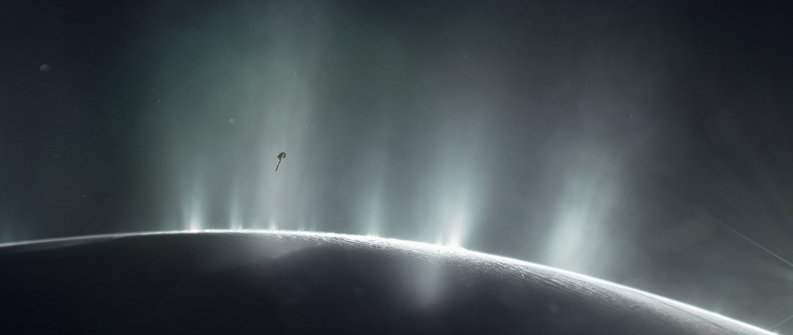
Surely we are not a special case; if life could get started here and chemistry is the same everywhere in the universe, then the factors that led to life here (whatever they were) are likely to occur elsewhere. Life could be abundant in the universe. That isn’t to say that intelligent life is abundant; on Earth, conditions may have been just right for us to evolve intelligence (more on this in our next edition). But once life gets started on a planet, according to how tenacious life has been here through six major extinctions, it is likely to hold on; perhaps even in our own solar system, on Mars, or Enceladus, or Europa. If we can get remote instruments out to these 21 star systems, we may very well find life.
I for one hope that some day a form of faster-than-light travel can be realized, perhaps even something like a warp drive in Star Trek. I hope life is as common as science fiction hypothesizes. It would be a wasted universe if we are the only ones out here.
A painting of an exoplanet by one of my students at New Haven School. We followed tutorials for using spray paint to create exoplanet images.
My first planetarium software was an old black and white program that ran on a Macintosh Classic computer. I have tried to find a reference for it, but can’t remember its name. As a physics teacher at Juab High School in the small farming town of Nephi, Utah in the early 1990s I had access to a 10” reflecting telescope on a broken down equatorial mount with a burnt out motor. I set up a few evening star parties for students and used the old software to find the locations of the planets and interesting stars and nebulas. We had to move the scope by hand, but it worked all right.
While working through a unit on astrophysics, I came up with a wild idea: to have students create a model of the nearby stars out to about 15 light years. I of course had heard of Alpha Centauri (I grew up watching the original Lost in Space) and had read enough science fiction to know that Tau Ceti and Epsilon Eridani were also nearby stars, but that was about the extent of my knowledge. It became a research quest of mine: to find a table of the nearby stars. I scoured my old college astronomy textbook and it had a table of the brightest stars, but not the closest, although it did list some of them such as Sirius. I looked in university libraries and began to piece a list together. Now this was 1993, and the Internet as we know it now was only beginning. In fact, Tim Berners-Lee developed the World Wide Web system with hypertext about that time, so research had to be done the old way, using the Dewey Decimal System and library index cards.
A spray painted illustration of exoplanets by Terrin.
I finally put together a moderately complete list and developed my own lesson plan activity. Our first attempt used a large styrofoam ball in the center and the stars were beads glued on wooden skewers poked into the ball. Measuring the right ascension and declination was difficult, and the final model was not very accurate or complete. The next year my lesson improved – we hung the stars from the ceiling with black bulletin board paper around and strips of tape for the Vernal Equinox and Celestial Equator, using a primitive sextant to get the angles and proportional spacing correct. We got the stars mostly hung before I realized we had them backwards, so we tore it down and started over. Right Ascension had to be measured to the left, it turned out. It was a great improvement, but the stars were various sized styrofoam balls and didn’t hold up well with repeated use.
Over several decades of teaching and through different schools, I revived the nearby star model every time I taught astronomy. Finding a place to hang it was a challenge. I decided that it would be better to create a hanging platform that could be attached to eyebolts in the ceiling using painted wooden balls on black string and black fabric hung around the model. Much better! I wrote up my lesson plan and submitted it for publication to The Science Teacher, and it was accepted with considerable editing and appeared in the Summer 2014 edition. I even taught this lesson plan at the Jet Propulsion Laboratory through my role as the Educator Facilitator for the NASA Explorer Schools program. The original activity expanded into a complete unit on the nearby stars.
Meanwhile, this full-scale hanging platform model was too big to take on the road, so I designed and built my own tabletop model using foamcore as the hanging platform (now actually the lid of a box) and trigonometry to measure the lengths of the strings for the stars to make the final model more accurate. I took this model to several conferences and presented it, but over the years the tape yellowed and lost its adhesion and there were new stars (brown dwarfs) discovered. The positions of all the stars were more accurately measured by the Hipparcos and Gaia space probes, so that my model was falling apart and needed to be upgraded.
My own attempt at spray painting an illustration of exoplanets.
This past summer of 2020, my astrobiology class spent a week building a new tabletop model. We used the Wikipedia article on the nearby stars (so much easier than the first time) and teams created a spreadsheet to calculate the scale distances needed to hang the stars in the model using trig functions. They drew in scales on the model and calculated where to poke the holes in the top foamcore. Other teams measured the strings, or created the labels, or painted the wooden beads. Then teams of three students each came up and hung one star system at a time in the model, starting with Sol and moving outward. We used a scale of one light year equals 2.5 cm. Now I have the model stored in my room and use it for every astronomy class. This summer my astronomy students built scale 3D models of various constellations, which is an easier activity as I only have them hang the most prominent 6-8 stars.
This quest to find out the names and positions of the nearby stars has served me well, as it has led to many opportunities to teach other teachers and students about the night sky. At the time I started this in 1993 no one was really talking about the nearby stars; then the first exoplanets were discovered such as Beta Pictoris b and the 55 Cancri system. Now it has become a hot topic. I have published other lesson plans for how to measure the distances to stars using parallax or my constellation in a box activity previously on this site.
Our model of the nearby stars out to 15 light years. We used trigonometry to get the vertical distances of the stars from the top of the model.
This third edition of Ad Astra will feature articles on the nearby stars and exoplanets, including basic information about the more interesting nearby stars. My astrobiology students last year wrote most of the articles that are included here. Where articles were not completed or the particular star system was not chosen by a student, I will fill in the gaps.
When, as teachers, we get the unavoidable question “Why do we have to learn this stuff?” my answer is always the same: the stars are out there, every night. Students might not be able to see them very well because of light pollution, but I grew up in a dark sky area a long way from any city in the west desert of Utah, and the stars are my friends and I longed to visit them. It would be a shame to go through life without any knowledge of them or how they have influenced humanity from our fundamental mythologies to our current technologies. Ignorance is not bliss. Ignorance is weakness; those that don’t know things can be easily controlled by those that do. I can’t imagine going through life ignorant of the universe around me. One may say that having a knowledge of the stars detracts from their romance and mystery. On the contrary, the more I learn about the stars, the more fascinating they become. I can look at a star and say that I know exoplanets are orbiting it, some in the habitable zone. There could be life up there. I can say that we can’t even see most of the stars (and they don’t show up in planetarium software) because they are too small and dim to be seen by our unaided eyes. I know the tales of the constellations, the ancient myths behind history. I am at home among the stars. “Though my soul may set in darkness, it will rise in perfect light; I have loved the stars too truly to be fearful of the night” (Sarah Williams, 1936, The Old Astronomer to His Pupil).
A hand drawn illustration of an exoplanet by Kat with a supernova remnant added in the background.
As a member of a choir at my university, I learned the music to Robert Frost’s poem “Choose Something Like a Star.” The narrator of the poem expresses frustration at how taciturn the star is; it says nothing about what elements it blends, or at what temperature it burns. But Frost was wrong; as much as I like the poem, stars do tell us all about themselves. From their color and spectrum we can tell what elements they blend, what temperature they “burn” (technically fusion), how fast they move, even if they have invisible planets orbiting around them. We have learned to tease a great deal of information out of the light they emit. In the end, the poem comes to peace with the knowledge that the stars are steadfast friends, reliable and ever present, something we can count on. In this world of uncertainty, that means a great deal.
O Star (the fairest one in sight), We grant your loftiness the right To some obscurity of cloud— It will not do to say of night, Since dark is what brings out your light. Some mystery becomes the proud. But to be wholly taciturn In your reserve is not allowed. Say something to us we can learn By heart and when alone repeat. Say something! And it says, ‘I burn.’ But say with what degree of heat. Talk Fahrenheit, talk Centigrade. Use language we can comprehend. Tell us what elements you blend. It gives us strangely little aid, But does tell something in the end. And steadfast as Keats’ Eremite, Not even stooping from its sphere, It asks a little of us here. It asks of us a certain height, So when at times the mob is swayed To carry praise or blame too far, We may choose something like a star To stay our minds on and be staid.
Robert Frost, 1916
Here is the completed 3rd edition of our Ad Astra per Educare magazine. I hope you enjoy it and share it. This post has been my editorial article taken from the magazine. Future blog posts will include the articles by my students and the longer feature article on the nearby stars. Things have certainly come a long way from that initial newsletter I had my digital media students create using Quark XPress way back in 2000. We’ve found out so much more about the nearby stars since then including whole new stars and 13 or so exoplanets within 13 light years of Earth. More will be discovered. It is nice to see this topic of the nearby stars finally coming into its own.
Dr. Rakesh Mogul of NASA’s Office of Planetary Protection and the CSU Spaceward Bound program
This interview was recorded in March 2012 while I was a participant in the Spaceward Bound program for teachers in the Mojave National Preserve near Baker, California. Dr. Mogul brought a team of pre-service teachers from the California State University system to do field research in the Mojave Desert. We collected biological soil crusts (BSCs) at three sites in the desert along Kelbaker Road and studied them in the laboratory at the CSU Desert Studies Center on Zzyzx Road.
David Black:
How did you become interested in science and specifically in astrobiology?
Rakesh Mogul:
I have always had an interest in science ever since I was a young kid. And I think it must have been pictures of astronauts and pictures of spaceships on my school classroom walls that got me into NASA, think- ing about what it means to be an astronaut, what it means to discover life and other types of chemicals in outer space. I’ve had an interest in this stuff since I was a little kid, very little kid.
David:
So what pathway did you take to get from high school up to working for NASA?
Rakesh:
It was a bit circuitous, really, I took the traditional route of basic science. I got an undergraduate degree in chemistry, a PhD in organic chemistry with a research emphasis in biochemistry, or protein chemistry, or chemical biology, depending which way you want to define it. And then I did a postdoc and I got a lecture position and I was got my first academic job and basically pure organic chemistry, biochemistry. I always had the NASA thing kind of in my back pocket. And finally, I had a chance to apply for a fellowship to go to NASA and I got the fellowship and ended up at NASA Ames Research Center for two years in the early 2000s. And that was my first real major endeavor into the NASA sciences and I’ve just been continued ever since then.
The Perseverance Rover with major instruments
David:
So what sort of things have you done at NASA?
Rakesh:
I worked with plasma sterilization and the bio- molecular effects of low temperature plasma such as CO2 plasma and O2 plasma, was on biomolecules and certain microorganisms, also did some work on bio nanotechnology using engineered proteins from extremophiles. And in more recent history, I’ve been working with extremophiles isolat- ed from the assembly facilities, where they build spacecraft. These microorganisms are found in these facilities, and are tolerant to the conditions found in the clean rooms. So what we do in my lab is some entomology, some proteomics and some remote microbiology, on these microorganisms. Basically we’re trying to study why they are resistant to things like hydrogen peroxide or ultraviolet radiation.
David:
So right now you’re working with the Office of Planetary Protection, but explain what that office does and what its role is.
Rakesh:
The Office of Planetary Protection’s primary role is to minimize the biological contamination of the solar system that may result from human based exploration – robotic exploration and basic human exploration. So these type of things involve correct fly paths to planetary bodies of interest, and especially the sterility and the cleanliness of the spacecraft that goes study the surfaces of planets such as Mars and maybe Europa in the future and Enceladus. In a nutshell, that’s planetary protection.
The Office of Planetary Protection’s primary role is to minimize the biological contamination of the solar system that may result from human based exploration.
Rakesh Mogul
David:
So what are the protocols or some levels of protection used by the Office of Planetary Protection to determine if a certain space probe or a certain mission is going to need to be highly decontaminated?
Rakesh:
There are different categories for missions, categories one through five, depend- ing on where the mission is going, what the target location is. So if you’re going to Earth’s moon, there’s really no sterility requirements. There are some requirements. For example, cataloguing the number oforganic molecules, organic compounds that might be on the spacecraft, but there are no cleanliness or sterility requirements beyond that for things such as Venus and Earth’s moon. But if you’re going to Mars looking for life and looking for signs of habitability, there are certain dimensions that have to be met. Those dimensions include the number of spores per meter squared, and the total spores found on the spacecraft. So these are the types of things that are considered. There are also a number of probability factors, for example, the impact probabilities and contamination probabilities that must be calculated out for planets such as Mars and icy satellites, such as Europa, and Enceladus.
What Mars may have looked like 3.5 billion years ago, when it had an atmosphere and oceans.
David:
So you essentially calculate what the risks are, and then communicate back to the missions what their sterilization protocols are going to be?
Rakesh:
Yeah, well, it’s more the mission’s responsibility to do the calculations and then to come up with a plan. And then they submit this stuff as a formal doc- ument called the Planetary Protection Plan. And they do this before the spacecraft is really assembled, and before launch ever occurs, and then that is approved or modified by the Planetary Protection Officer. And then it goes back and forth until they agree on something and then they move forward. And so there it’s not so rigid. The requirements are there because there are requirements, but if you can’t meet them, there are certain ways around them. There are waiver requests, there’s sometimes alternative methods to bring the bioburden down or to reduce the impact or probabilities or to reduce the impacts of contamination.
David:
Alright, so we have the Mars Science Laboratory on its way to Mars. Obviously, since it’s also going to be trying to detect organic molecules, the protocols here have to be really high. So what are some of the methods that were used to sterilize or decontaminate MSL?
Rakesh:
So, MSL was not, did not undergo full system sterilization will they sterilize the entire spacecraft all at once. They kind of haven’t done that in a long time. But they had to clean certain parts with ethanol and isopropanol, kind of cleaned it off and made sure the bioburden was quite low. I believe a few parts may have been sterilized by vaporous hydrogen peroxide, but I’m not confident of that one, they may have been so. And maybe a few parts, just tubing and I forgot the other examples – I think there were one to two or three parts that they did sterilize via dry heat microbial reduction, or DHMR. They use a variety of things. And it was all basically depending on the type of material that they’re going to sterilize and where it was.
What Jezero Crater looked like 3.5 billion years ago. As a crater filled with fresh water, it had both inflow channels with deltas and an outflow channel. Water was here long enough that if Mars had life, this would be a good place to look.
David:
So taking the material from the robotic arm, which is taking regolith back to the SAM instrument, obviously, the arm has to be decontaminated.
Rakesh:
Yes, and it was a category 4A mission, so they’re not looking for life. And they’re not really looking for that many hardcore signs of life. So their sterility requirements were probably the least stringent for going to Mars for landing on Mars. So there’s differ- ent levels of sterility, if you will, or cleanliness for a Mars mission that lands on Mars and rolls around or just stays put. And those different categories are 4 A, B, and C. And MSL is 4A, where Phoenix was a 4B, and Viking, the equivalent would be 4C.
David:
How did you get involved with Spaceward Bound?
Rakesh:
I heard about Spaceward Bound somewhere between 2006 and 2007, from a colleague of mine, and I had known Chris from my prior days at Ames Research Center. So I simply emailed Chris out of the blue asked about the program and asked if I can participate in some form or another. And he wrote back almost immediately and said, Yeah, come on by and participate. So as the first year I came, I was just a participant, like many people here come for the first time, I didn’t have any science plan. And I came up and I just got a real good introduction to what field science is. And up until that point, all of my work was in the lab. Even if those were NASA related it was always in the lab. And I had done no field work and had no experience with field work all throughout graduate school, my academic career, and through my time at NASA Ames. Always an in the lab guy, in vitro, if you will. And so my first Spaceward Bound was my first introduction to field science. The next year, I came back as part of the science crew. And I was doing actually then redox essays on the soil crusts, and different soil communities around here looking for bulk properties of reduction or oxidation. And then the following year is when I started this program, then involved the CSU undergraduates and master’s students. And ever since then, we’ve been running this program.
Dr. Mogul was kind enough to allow me to interview him for about 45 minutes on the last day of our Spaceward Bound field study in the Mojave National Preserve.
David:
So a combination of students come in from CSU, scientists from NASA and other places, all combining together to do field research with a desert focus.
Rakesh:
Yes, that’s exactly right. And to add on to that the fundamental point to Spaceward Bound as it’s evolved with the CSU, the California State Uni- versity system, is basically a program designed to bring pre-service teachers, basically teacher wan- nabes, who are undergraduate and or master’s students and bring them out to the desert to give them (A) an introduction to astrobiology, (B) an introduction to field science, especially it relates to astrobiology, and then (C), most importantly, to give them hands-on experiences with doing real science in the aspect or concepts of NASA.
David:
So why study soil crusts?
Rakesh:
Soil crusts are surface communities and microorganisms that live in a symbiotic manner. So it is a simplistic form of a multicellular community that is very intrinsically dependent on the health of each one of the members. So it does relate to early forms of life. So when microbes all live by themselves eventually live in symbiosis communities, and many of these are known as stromatolites and microbiolites. So I would believe that it might be that the biological soil crusts are another form of that. They are also found in semi-arid environments and arid environments, which means they’re quite temperature resistant, quite resistant to ultraviolet radiation, and they are quite resistant to desiccation. So they are potentially very good analogs for surface communities that may be found on Mars. They may not be found on Mars, maybe they were at some point. So it’s still a very good thing to study.
A drawing of Mars made by Percival Lowell for his 1906 book Mars and Its Canals. He saw lines across the surface, an optical illusion created by the eye’s attempt to connect the dots of craters. He thought the lines were canals dug by Martians. Now we have sent the Perseverance Rover to find out if there ever were Martians, or at least microbes.
David:
At least how they grow similarly to how things might grow on Mars.
Rakesh:
Correct. Correct. High UV environment, dry, and not connected to any vegetation. And very much dependent on – they’re very much a critical member of the health, if you will or fertility of soil. So as the BSCs go, so does it refer to the fertility of the soil.
David:
Just kind of like a barometer.
Rakesh:
They are definitely a barometer. If the biological soil crusts are dying, that means the land itself is not so fertile and that comes back to the water retention that they add to the soil properties and the carbon and nitrogen and recycling.
Dr. Matt Golombek was the Project Scientist for the Mars Pathfinder mission and now chairs the Mars Site Selection Committee
The first time I saw the movie Hidden Figures was under unusual circumstances. I was presenting a poster at the Lunar and Planetary Science Conference along with two students in March 2017. The conference is held every year near Houston in the Woodland Hills Convention Center, which is across the street from a large shopping mall and theater complex. The conference rented out a special showing of the movie just for conference attendees, so we decided to go. It is always fun to see a science-themed movie with knowledgable people. This audience gave the biggest laugh at the part where Octavia Spencer, acting as Dorothy Vaughan, finds a book that states on its cover that FORTRAN is easy to learn. We all knew better.
This is a context view for Tooting Crater on Mars, rendered from 3D MOLA data and showing the larger area of Olympus Mons and its lava flows.
As we were standing in line for the movie, a man came and stood in line behind us. I turned around and saw that it was Dr. Matt Golombek, Project Scientist for the NASA Pathfinder/Sojourner mission and co-chair of the NASA Mars Site Selection Committee. He has been in the middle of selecting the landing sites for our missions to Mars since Pathfinder landed in 1997. I met him previously when I helped to plan and implement an educator workshop at JPL in 2002; we invited him to speak to the teachers about his experiences with Pathfinder and with selecting landing sites on Mars for Spirit and Opportunity.
Tooting Crater, just to the left of the lava flow. The smaller hole nearby is an exposed lava tube, and the ejecta from the crater appears to have splashed. The flat orange area was an ocean basin. These are all good reasons to send a rover here to look for signs of life.
I said hello and acknowledged that he was having a very busy year. He told us that the committee was working on deciding three different landing sites that year: one for the InSIGHT lander that would finally be traveling to Mars the next year, one for the Mars 2020 rover (since named Perseverance) and one for the European Space Agency’s Franklin Rover, both scheduled to launch in 2020. The 2020 rover had had its landing sites narrowed down to three candidates by the time of that conference, and large posters were up in the convention center showing the sites using 3D imagery from the Mars Global Surveyor MOLA data and the Mars Reconnaissance Orbiter’s HiRISE camera.
The finalist sites were to return to the Columbia Hills in Gusev Crater, where signs of a hydrothermal vent had been discovered; an area at the northeastern edge of Sirtis Major where there were many river channels leading down into Isidis Planitia; and Jezero Crater, also at the edge of Sirtis Major where there were large delta deposits and a nice flat landing area nearby.
A context view of the large river channel flowing from the north rim of Argyre Planitia northward toward Ares Valles. It passes through several craters. Holden Crater is the largest at the top center, just past where Nirgal Vallis enters the channel.
There are a number of challenges in choosing a landing site. It must be flat enough for a safe landing, without major boulders or craters or slopes that might spoof the radar landing system. It must be close enough to areas of high scientific interest that only a short drive is necessary to reach them, or ideally the landing ellipse is right on top of areas of scientific interest so the rover can go to work immediately upon landing and instrument check-out. If it has solar panels, then it needs to land near the equator to have enough sunlight and to survive martian winter. If it has RTGs (radio-thermal isotope generators – a type of thermocouple powered by the heat from the radioactive decay of plutonium) such as Curiosity does (as well as Perseverance), then it can land further from the equator and survive longer. It needs to land at a mid to lower altitude site so that aerobraking and parachutes can slow it down sufficiently for the sky crane to work. And it needs to not be near any obstructions that could prevent it from relaying data through the several orbiters we still have at Mars.
Holden Crater close up. The river channel comes in from the left and leaves a delta deposit; the indentations at the top are amphitheater erosion patterns with alluvial fans, similar to what you see along fault zones in the Great Basin of Utah.
With the site selection committee that Dr. Golombek heads, scientists suggest sites for landing based on the suite of instruments of each mission and what its goals are. Those suggestions are discussed and debated back and forth by the scientific community, with some eliminated and others added. Detailed maps and images, complete with mineralogy, are created by multiple passes over the sites with our orbital probes. Gradually the best sites rise to the top of the discussions and the choice coalesces around a final few. The committee than debates and chooses the final site.
A mineralogical map of the delta deposits in Jezero Crater, showing an abundance of phylosilicates (clays) and other sedimentary deposits that are ideal for preserving signs of life. The rover is targeted to land just south of the delta in the flat area, a very short drive away.
For Perseverance, the site selected is Jezero Crater (my top choice as well). It launched this July and is now halfway to Mars, landing on Feb. 18, 2021. Technically, the spacecraft is slowing down as it heads outward from the Sun; it will reach a point where Mars will intersect with it on February 18th and hopefully have a bullseye landing right next to the delta deposits. The ESA Franklin Rover has been delayed until the next conjunction 26 months from now in 2023 due to issues with its parachutes not being tested in time for the launch because of the pandemic. The United Arab Emirates has launched the Al Amal (Hope) Orbiter, and the Chinese have launched an orbiter/lander/rover combination called TianWen-1. February 2021 will be a busy month for Mars exploration.
The orange area to the northwest of Deuteronilus Mensae is one of the landing sites selected. There are mesas with multiple old sedimentary layers, river channels, and recent dunes to explore.
Mars Site Selection Activity
An activity that I frequently do with my astronomy students as a means for getting them familiar with the geographic (Areographic?) features of Mars is called the Mars Site Selection Committee project. I have taught this activity many times to different groups of students and at workshops at science teacher conferences. I taught it to my astrobiology class this summer just as these Mars missions were launching. I thought it might be time to share it through my blog site and through our Ad Astra Per Educare magazine.
A close up of the Deuteronilus Mensae landing site selected by on eof my teams.
To do this properly, you need to have some large posters of Mars’ surface or be able to project an online map of Mars. I use large Mars MOLA data posters that I picked up at the Educator Resources Center for the Jet Propulsion Laboratory. At the time I was doing workshops for JPL (2002-2004), the ERC was located off site at the old Indian Hills Mall in Pomona but it is now onsite at JPL by appointment only. In addition to the MOLA data posters, they had a box full of Mars Global Surveyor posters from National Geographic. Here is a source for a high resolution MOLA map:
I also have an old Viking era poster of Mars done by Silver, Burdett and Ginn that I found in the freebies discard bin of my local library – probably a collectors item by now and quite a find. I also use the MOLA 3D altitude data found at the Mars data page of the NASA Planetary Data System node at Washington University of St. Louis (choose NASA geosciences data and it will come up, then choose Mars on the list on the left, then Mars Experimental Gridded Data Record) as an online resource. Here is the direct link:
The highest resolution data is at the bottom of the page. If you are unfamiliar with using .img data, then I have a whole blog post (included further down this page) and a YouTube video on this at:
or you can use an already processed height-map of Mars in .tif format that is located here:
To actually run the activity, I describe the requirements for landing a rover on Mars and introduce students to the general features of Mars using my classroom and online maps. I show them the sites we have already landed at, such as Chryse Planitia, Utopia Planitia, Ares Valles, Gusev Crater, and Terra Meridiani. I show them renders of 3D terrains I have built of these sites and describe why we landed there and what we learned from each site.
On the eastern edge of Valles Marineris (at the center of this image) is a narrow channel where all of the Marineris outlfow passed through, providing long-term water erosion and sediment deposits.
I then propose a next generation Mars rover that has various mission objectives and instruments, and ask them as teams to pretend that they are representing the planetary science departments of universities and the principle investigators of each instrument. They are provided with maps or look them up online, then zoom in as much as possible to see specific features. They must find a site that has the following characteristics:
Here is a close up render of the same site. Flowing water carved a flat channel at the narrow opening, and chaotic terrain is within reach to the west.
It must be flat and level for an area about 50 km on a side.
It must be near areas of scientific interest. If the purpose of the mission is to search for signs of life, then the site must have evidence of long-term standing or running water with sedimentary deposits of clays or other minerals that would preserve evidence of fossils.
It must not be over 60 ° from the equator or the rover may not survive cold winters.
I allow the student teams some time to look at possibilities and I walk from team to team, describing any areas they are interested in and whether it meets the criteria. As they notice river channels, I provide names and point out features such as tributaries, meanders, deltas, etc.
The second day, the teams choose a final site and I use the .tif file at the link above, cutting it down to a medium sized image and a smaller image of the specific landing site. I then use the procedure listed on my blogsite to print 3D models of the teams’ terrains:
I then use the 3D model to create renders in my 3D software, adding a gradient texture that is altitude sensitive and printing out the final renders to the teams. The medium sized data becomes a context image and the smaller data becomes a detailed image of their landing site. The teams look up information about the site, as much as they can, and create a presentation using their renders and other images they find to justify why they want to land there, based on the criteria above.
The first team chose the lowest part of Valles Marineris, the deep magenta area in about the center of this 3D render we did using MOLA data.
The teams then present their case for the landing site, and all the students then vote for what they think is the best site.
For my summer astrobiology class, I had six teams and these are the sites that they chose:The lowest part of Valles Marineris at the entrance to Coprates Chasma. Lots of erosional debris is available here from canyon walls slumping. We could discover if the layers we see in the Marineris walls are volcanic or sedimentary.
A close up of the central part of Valles Marineris. The walls of the valley have slumped, carrying a great deal of geological history within reach of a rover.
2. Further to the east, where the Valles Marineris drains through a narrow canyon toward the chaos terrain and the start of Ares Valles. Water flowed here for a long time.
3. Holden Crater, on the drainage system from Argyre Planitia toward the north after Nirgal Vallis joins the channel. It has amphitheater erosion patterns and alluvial fans that speak of ice wedging and other erosional processes. There are also delta deposits, although it is a long drive between.
4. Tooting Crater, just to the west of Olympus Mons at the bottom of Amazonis Planitia. Their are interesting lava tubes and evidence that the ejecta from the crater was mostly mud because it left splashes that flowed, not the usual dry ejecta pattern. It is also close to the cliffs of Olympus Mons that would have been sea cliffs when this was an ocean bed.
To the right and up from the center of this 3D render is the landing site selected by the Hellas Basin group. There are riverbeds and other evidence of long-term water.
5. The northeastern edge of Hellas Basin, where a number of river channels drain down toward the bottom of the large crater.
6. Northeast of Deuteronilus Mensae and Sirtis Major, where there are eroded mesas of sedimentary deposits along with ancient clays and recent sand dunes. This was one of the final three sites for Perseverance.
A close up render of the Hellas Basin rim site. There are multiple river channels leading down toward the bottom of the basin and what appears to be a shoreline at the edge between the orange and yellow areas.
The final vote came out strongly in favor of Tooting Crater. The team did a good job of addressing all the criteria. Second choice was NE of Sirtis Major and third choice was Holden Crater. I hope scientists take an interest in Tooting Crater, as it really is an interesting site, given the lava tubes, splashed ejecta, and access to Mons Olympus volcanic deposits as sea cliffs. If we follow Elon Musk’s vision of a city on Mars, this would make a good site.
I think the activity went quite well, and it certainly fulfilled its major objective, which is to help students learn the features and geologic history of Mars.
Venus has a thick, toxic atmosphere made mostly of carbon dioxide and sulfuric acid. Yet phosphine gas, a biomarker on Earth, has been detected in the atmosphere.
Astrobiologists have yet to find conclusive proof of life outside Earth, although tantalizing clues of the possibility of life do exist. Just this week, researchers announced the discovery of phosphine gas in the clouds of Venus. Phosphine is found in Earth’s atmosphere and is mostly of biogenic origin, created by certain anaerobic bacteria. The phosphine on Venus is of too high a concentration to be easily explained by non-biogenic sources such as lightning; life could be a possible explanation, but that life would have to survive in an extreme environment, since the clouds of Venus are 96% sulfuric acid.
To understand what such life might be like, we study organisms on Earth that can survive and even thrive in extreme conditions, including high acid environments. These extremophiles are an analog of what we could look for on Mars, under the ice of Enceladus or Europa, or in the clouds of Venus. By studying extremophiles, we train ourselves how to study life elsewhere.
The following short articles were researched and written by students at New Haven School in Spanish Fork, Utah as part of their astrobiology summer course. Because privacy concerns, I am only providing their initials.
The surface of Venus is hot enough to melt lead, has a pressure as great as 26 Earth atmospheres, and rains sulfuric acid. You would die horribly four different ways if you stepped foot outside without a spacesuit.
Acidophiles by V. N.
An acidophile is a bacteria / animal that can or must survive in a highly acidic area. An acidic environment is an area that has a pH level below 6. An organism is only considered an acidophile if it can thrive in an area with a pH below 2, areas such as that are considered highly acidic. Acidophiles are able to survive in highly acidic environments due to their membrane system which pumps out protons into the intercellular space; the result helps keep the cytoplasm at or around a neutral pH. Due to this process it is not necessary for intracellular proteins to develop acid stability.
Certain acidophiles such as Acetobacter aceti utilize an acidified cytoplasm, this forces out nearly all of the proteins in the genome to get to acid stability. The Acetobacter is a great way to understand how proteins can obtain acid stability. Many studies focused on acidophiles have shown a few mechanisms by which the acidophiles obtain a steady amount of acid inside them. In most stable acid proteins there tends to be too much acid residue which affects low pH stabilization created by a buildup of positive charges. Other ways acidophiles survive is by minimizing the solvent accessibility of acid residues, or by binding the metal cofactors.
Acidophiles are incredible at adapting to harsh environments. It is notable that acidophiles can survive in an impressive amount of harsh and unwelcoming environments that humans couldn’t imagine or physically stay alive in.
Alkaliphiles by K. T.
Did you know harsh environments can sustain living organisms? These organisms are known as extremophiles. The definition of an extremophile is “a microorganism, especially an Archaean, that lives in conditions of extreme temperature, acidity, alkalinity, or chemical concentration.” (Dictionary, Definition of Extremophiles, google.com). Within extremophiles are classes, such as alkaliphiles. These species are known to grow around a pH of 10. Certain microbes qualify as this specific class.
An alkali bee with nesting hole. These bees thrive in highly alkaline soils, with pH around 10.
Alkali bees are a suitable example for an animal that can survive a harsh environment. Alkali bees dig nests underground looking for salty soil, this is categorized as an haloalkaliphile. They create a strategic arrangement of tunnels to lay eggs in safety. Their lifestyle is isolated and not livable for other creatures, but they adapt to it quite easily, since it is in their nature to do so (Alkali Bees, fs.fed.us.com).
Other categories known are the obligate and facultative alkaliphiles. Obligates require a very high pH to survive, and facultative are able to survive in high pH climates, but also are adaptable to normal conditions (en.wikipedia.com, Alkaliphile). Alkaliphiles are still currently being discovered and not very much is known about them in this present day. Even though there is little information, the research continues to explore more about the adaptations and creatures surviving under these harsh, unlivable climates.
Clostridium by S. E.
Clostridium is an anaerobe, a type of extremophile which can survive without oxygen, metabolizing on their own without external energy (oxygen). They are also a genus of Gram-positive bacteria, which means they change into a certain color when exposed to a staining method introduced in 1884 by Hans Christian Gram. Clostridium is commonly known in the medical world because this specific type of anaerobe is known to cause and accelerate human pathogens by infecting the intestinal and digestion tracts by overproducing healthy fiber, overloading the dietary system; often appearing as Clostridium perfringens (food poisoning) or Clostridium tetani (tetanus) in the body, this genus can cause many infections which, like the latter condition of tetanus or lockjaw, can sometimes be fatal.
Clostridium frequently exists in airtight containers, as it is able to survive anaerobically, or without air, causing food poisoning to those who eat canned goods infected by this anaerobe. A prokaryote, or a bacterium lacking sophisticated internal systems, Clostridium is sometimes classified as a disease. As for anaerobes in general, other substances and energies than oxygen are used in metabolism and respiration, such as nitrates. They do best in regular body temperature environments, unlike other extremophiles which can survive in severe temperatures.
Clostridium, a type of anaerobic bacteria that can thrive without oxygen in airtight containers. If it gets into foods, it will produce toxic byproducts that cause food poisoning.
Clostridium strains cause disease and infection by secreting toxins in lysis, the organelle process in which the cell membrane is ruptured by viral infections. In closing, Clostridium is a bacterium, often rod shaped, and the cause of toxins that can be potentially fatal and are often very resilient due to their status as anaerobes.
Halophiles by N. D.
Halophiles are a type of extremophile that thrives in environments with high concentrations of salt. The name “halophile” comes from the Greek words “salt loving.” Halophiles mainly live in evaporation ponds or salt lakes. Some examples are The Great Salt Lake, Owens Lake, and the Dead Sea. Those bodies of water contain a salinity of 33.7%. That’s about 10 times saltier than any ordinary seawater. That amount of salt allows halophiles to thrive in their environment.
Halophiles are chemoheterotrophs, using light for energy and methane as a carbon source under aerobic or anaerobic conditions. Halophiles contain proline, amino acid derivatives, polyols, sugars, and methylated sulfur compounds. Halophiles are a very complicated and detailed organism that is difficult to study. Most halophilic and other salt eating animals use energy to remove salt from their cytoplasm. Normally, organisms living in salt would lose water and die because of osmosis—other than halophiles.
The Spiral Jetty in the north arm of the Great Salt Lake. The pink color of the water is caused by a halophilic bacteria that stains the water pink.
Halophiles are categorized by the levels of salt on which they grow best: slight halophiles, moderate halophiles, and extreme halophiles.
Hyper Piezophiles by L. M.
Hyper Piezophiles are organisms that survive and reproduce in high pressures in the depths of the ocean or deep underground, also known as the deep biosphere. In order for these organisms to live in these extreme environments they develop various mechanisms to prevent the effects of the elevated pressures they live through. They live more than 1000 m below sea level, which has a hydrostatic pressure greater than 10 MPa. In the deep biosphere there is lack of light and nutrients and very little organic materials.
When piezophiles are isolated they can be divided into thermopiezophiles and psychropiezophile. Pyroccus yayanosii strain CH1 is the only known thermopiezophile and is found in hydrothermal vents. Hydrothermal vents are splits in the ocean’s floor where water is geothermally heated up to 400°C and emitted and then results in eutrophic, microbial dense communities. Psychropiezophiles are found in the depths of the ocean also, but in areas that are not heated by geothermal energy that reaches about 2°C.
Osmophiles by B. H.
There are probably a lot more creatures living in your food than you think. Osmophilic organisms are adapted to live in areas with high sugar like jam or honey. The adaptations that osmophilic organisms have are they can make glycerol to balance their internal and external osmotic pressure. They can also shrink their membranes to keep the glycerol in their cells. Yeasts are common osmophilic organisms you might discover in foods containing high amounts of sugar. Some types of yeast, molds, and bacteria are osmophilic.
Osmophilic organisms are some of the only organisms that are adapted to live in high osmotic pressures. A lot of different foods have sugar in them because the sugar will suck up all the water around it, making it a great food preservative. I don’t know about you but I know that now I will look at food totally differently and will be more careful about what I eat. I don’t want to get sick or even risk getting sick. The bacteria that lives in your food can be either good or bad; be sure you are not eating a bunch of bad bacteria.
Too Hot to Handle: The Weird World of the Pompeii Worm
by J. W.
The Pompeii worm lives at hydrothermal vents in the deep ocean under high pressure, with extreme heat at its head and cold at its tail
Imagine living comfortably in 140-degree water. Seems impossible, right? Not for the Pompeii worm. Discovered by marine biologist Craig Cary and his colleagues in 1997, the Pompeii worm (scientific name Alvinella pompejana) is a species of deep-sea polychaete worm, or “Bristle Worm.” Pompeii worms can reach up to 13 centimeters in length. They have a feather-shaped head and tentacle-like gills, colored red by hemoglobin. Pompeii worms live in tubes near “black smokers” — hydrothermal vents on the Pacific seabed that emit a substance comparable to black smoke. These worms are extremophiles, organisms that can live comfortably under multiple extreme conditions. For the Pompeii worm, those conditions are extremely high pressure and temperatures.
In fact, the Pompeii worm is known as the most heat-tolerant animal on Earth. Alvinella pompejana can survive at sustained temperatures of 105 ° C (221 ° F) for short periods of time, but it is most comfortable in temperatures ranging from 40 to 60 ° C (113 to 140 ° F). Pompeii worms like to keep a cool head– while they rest their tails in water with temperatures as high as 80 °C (176 ° F), they rest their heads in cooler water, at temperatures around 22 ° C (72 ° F).
The Pompeii worm’s abilities to withstand the heat are linked to heat-stable ribosomal DNA and a symbiotic relationship with bacteria. The worms have hairy-looking backs; these “hairs” are actually colonies of bacteria, which feed off of mucus secreted from glands on the worm’s back. This layer of bacteria can be up to one centimeter thick! The bacteria are thought to provide insulation for the worm, thanks to eurythermal enzymes that protect the bacteria– and thus, the worm– from extreme temperatures. It’s clear– no one can take the heat like the Pompeii worm.
Extremophiles: Snottites by S. S.
Snotticles hanging from the ceiling of a cave in New Mexico. The mucus-like material is created by an extremophile that lives in the caves without light and is chemotrophic.
Extremophiles are organisms that live in extreme conditions. An example of an extremophiles is Picrophilus torridus, it is a thermoacidophile adapted in hot acidic conditions. It was found in soil near a hot spring in Hokkaido, Japan. Snottites or Snoticles are another extremophile that are found in caves hanging from the walls and ceilings. They have the consistency of nasal mucus and look like drips. Snottites got thier name by Jim Pisarowicz in 1986. They get their energy from chemosynthesis of volcanic sulfur compounds including H2S and warm water solution dripping down from above. Because of this their waste is highly acidic with similarities to battery acid. Diana Northup and Penny Boston brought attention to snottites while studying in a toxic sulfur cave called Cueva de Villa Luz in Tabasco, Mexico. Northup says that at certain times of the year the slime makes the walls look like they have been silvered, she says that “it’s just breathtakingly gorgeous.” Some cave systems Snottites are found in are the Frassasi caves in Italy, Grotta di Rio Garrago, and Cueva Luna Azufre.
Tardigrades by S. W.
Tardigrades are incredible and extremely resilient microscopic animals. Although they look soft and puffy, they are actually covered in a tough cuticle closely related to that of a grasshopper. First discovered in 1773 in Germany by J.A.E Goeze, these tiny extremophiles were named “Kleiner Wasserbär” or “little water bears” in English. In the grand scheme of time, Tardigrades were discovered a long time after the start of their existence. Scientists have traced them back to roughly 4 million years before the oldest of our found dinosaurs.
As of today, roughly 1,300 species of Tardigrade have been found and can be properly classified each of which share some similar features. All Tardigrades have four to six claws on each of their eight feet used to easily allow them to cling to plant matter. They all have a mouth-like structure known as a buccopharyngeal apparatus used to suck in nutrients from plants and other microorganisms.
A tardigrade, or little water bear. These microscopic creatures like wet, mossy environments but can survive extreme dryness lasting years by rolling into a ball which preserves moisture. They are protected from radiation by a layer of protein on their cuticles.
Tardigrades have been nicknamed “Moss Piglets” due to their preference to live in mossy areas with lots of fresh water moisture and their slight resemblance to tiny, grey pigs. Although they prefer wet areas, Tardigrades have been proven to thrive even in desert sand dunes because they keep an extremely thin yet useful layer of water around their bodies at all times. Because they keep themselves moisturized so well, Tardigrades can actively survive without food or water for up to thirty years.
Tardigrades have incredible resilience to many different substances. They have a unique protein in their bodies called a Damage Suppressor or “Dusp” in shortened terms. This amazing protein protects them against extreme radiation which can be present in soil, water and around plant life. These damage suppressing proteins also allow them to survive at a temperature of up to – 328 ° F (- 200 ° C) or beyond boiling, in pressures six times harsher than in the deepest of our ocean’s trenches and they can withstand the cold vacuum of outer space for an impressive amount of time. Although it may seem so, these tiny superbeings are not immune to everything. They are very sensitive to acidity. Even the lowest levels of acidity can kill them almost instantly.
Known also as “masters of cryobiosis,” Tardigrades can practically freeze themselves in time and wait for unsafe conditions to pass by. Cryobiosis is a state of complete inactivity triggered by a lack of moisture. Tardigrades can squeeze themselves into tight balls tucking down their heads for protection. This allows them to release moisture through their skin like a living microscopic sponge. When their surrounding conditions improve, Tardigrades can quickly consume moisture and revive themselves.
Thermophiles by C. L.
Alicyclobacillus acidocaldarius are a thermophile species. These creatures can inhabit an environment with a higher temperature than most species can survive in. The first species of alicyclobacillus were found in the geysers in Yellowstone National Park, and also found in fumarole soil, which is an opening near a volcano in which hot gasses come out. They can be found in Hawaii’s Volcano National Park. Scientists decided that it should be classified as Bacillus acidocaldarius in 1971, then later on figured out that studies showed it to be from a different and new species called Alicyclobacillus. They live in acidic and high temperatures. Thomas D. Brock was one of the first scientists to categorize this species. The temperature in which Alicyclobacillus can grow at is 60-65 ° C, and optimum pH it can grow at is 3.0-4.0, which is a significant amount of acid. Over time they have adapted to the high acidic levels of their environments.
Grand Prismatic Spring in Yellowstone National Park. The rainbow of colors is created by different species of thermophilic bacteria that can live in the varying temperatures and high acidity of the water.
Hyperthermophiles by R. R.
Hyperthermophiles were first discovered by Thomas D Brock in 1965, isolated from the hot springs in Yellowstone National Park. There are now 70 species of Hyperthermophiles. The most extreme living on the walls of deep sea hydrothermal vents, a place one would normally see as impossibly habitable. What gives hyperthermophiles this incredible ability to endure and even thrive at such high temperatures actually has something to do with their protein molecules and cell makeup. Their protein molecules, which show hyperthermostability, allow them to maintain structural stability and function at high temperatures. These evolved hyper thermostable proteins allow chemical reactions within the organism to proceed faster at higher temperatures. Hyperthermophiles also contain high levels of saturated fatty acids in their cell membranes which allow them to retain their shape at their preferred temperature.
Hyperthermophiles live in hydrothermal vents, which are created by volcanic activity and tectonic plate movement. It is a fissure on the seafloor from which geothermically heated water comes from that can reach temperatures above 700 °F in some cases. There are two types of hydrothermal vents, black smokers and white smokers. Black smokers emit particle laden fluid that are made up of fine-grained sulfide minerals formed when the hydrothermal fluids mix with the very cold sea water surrounding the vents. White smoker vents have lighter minerals emitted and lower temperatures than that of black smoker vents. The mineralized fluids from this type of vent are rich in calcium and sulfate-rich and form carbonate deposits. Any creature able to withstand and thrive in such an environment is astounding.
3D printouts of sections of Mars using the Mars MOLA terrain data from NASA’s Planetary Data System Geosciences Node. The sections are, from upper left clockwise: Kasei Valles, Gale Crater, north of Argyre Planitia with Holden Crater, Mons Olympus and Tharsis Plateau, and Jezero Crater.
As a teacher or Mars enthusiast, have you ever wanted to 3D print custom Mars terrains? For example, as the Mars 2020 Perseverance rover prepares to land in Jezero Crater on Feb. 18, 2021, would you like to print out a 3D model of the crater or other places on Mars? This post will teach you how to do just that using a recent version of Adobe Photoshop, an online 3D program called SculptGL, and your favorite slicing and 3D printing software/hardware.
I have written previously about using Mars MOLA altitude data in your science classroom. To get the highest resolution .img files of Mars into a usable format for printing, I recommended using a small utility program from the National Institutes of Health called ImageJ, which allows you to open the .img files and resave them in various formats if you know the exact pixel dimensions and bit depth of the data. I have created a video of the first version of this process using ImageJ on my YouTube channel created three years ago; it can be found at: https://youtu.be/kzdO9PANu_8.
The NASA webpage for the Mars MOLA data. It is part of the Planetary Data System (PDS) Geosciences Node at the Washington University in St. Louis. You want to select the Mission Experimental Gridded Data Records (MEGDRs) link.
I have recently purchased a new Mac computer running MacOS 10.15 Catalina, and have not found a way to get ImageJ to work on this machine (if you know how, please let me know). I have purchased updated Adobe software including the newest version of Photoshop and have experimented with methods for getting the MOLA data into a 3D model using Photoshop’s new 3D features. It cannot read the .img MOLA data files directly, so I have had to use another source. The results have been good, although I have usually had to run the models through another program to flatten the vertical exaggeration and provide a supporting base before I can successfully print them on my 3D printer.
The high resolution MOLA data grid, at 128 pixels per degree or about 1 pixel every 30 meters. For 3D printing, you will want to use the Topography data. Each quadrant is named by the latitude and longitude of its upper left corner. The grid itself shows the coordinates of the upper left and lower right corners. You will need to look at the .lbl metadata file to see the exact number of data points for rows and columns and the bit depth (16 signed) for each pixel in order to open it in ImageJ.
This post will work you through the steps, including where to find the data, how to turn it into a 3D model, and how to prepare it for printing. The end results, when printed with color-changing PLA filament, have been quite successful.
Step 1: Finding the Data:
The high resolution MOLA data is located at the Planetary Data System Geosciences node at the Washington University of St. Louis (WUSTL) at this website: https://pds-geosciences.wustl.edu/missions/mgs/mola.html. You will need to click on the Mars Experiment Gridded Data Record (MEGDRs) link to get to the actual data, then scroll down to the bottom of the page to find the highest resolution data set, which is 128 pixels per degree on Mars, or about one pixel every 30 meters. The best data for 3D printing will be the topographic data, or files beginning with “megt.” The numbers after give the the latitude and longitude of the upper left corner of the section, so you will need a map of Mars to know what area you want to download. For the MOLA data, Mars has been divided up into a a 4 x 4 grid with 16 sections. Clicking on the megt-.img file you want will start the download process. These files are fairly large, so it will take a few minutes.
Web page for the lower resolution full Mars data. If used in Adobe Photoshop, the file will have a bi-gradient problem due to elevations lower than martian “sea level” having a negative value. This problem is easily fixed.
This map has a resolution of 463 meters per pixel but is still good for 3D printing. The colored prints of Jezero Crater, Tharsis Palteau, Gale Crater, Kasei Valles, and north of Argyre Planitia came from this image and had to be reduced in size even more before printing. The file is a 2 GB .tif, and if loaded into Adobe Photoshop will show a bi-gradient problem that I will discuss how to fix below.
Step 2: Loading and Converting the Data:
To use the data in ImageJ, you will need to look at the megadata file, or .lbl file. It will tell you that each grid has 5632 rows and 23040 columns and that the data is 16-bits per pixel and signed, meaning that there is an arbitrary “sea level” in the data with positive and negative values above or below that line. Once the .img file is downloaded, it can be loaded into ImageJ using File-Import-Raw. Choose the file you have downloaded, and it will then ask you for the columns (23040 in the newer data, 11520 in older versions) and rows (5632). Choose “16-bit Signed” from the Image Type pulldown menu, 0 for the offset, 1 for number of images, and 0 for the gap. Leave all the checkboxes at the bottom unchecked and click OK. Your section of Mars will then load and show as a grayscale heightmap. You can then save the file as a PNG.
Menus in Adobe Photoshop for converting a grayscale image (such as the MOLA data) into a 3D model. Choose “Solid Extrusion” from the final menu.
Step 3: Creating a 3D Model:
Using MOLA data through Image J: The file will be too large for most 3D printers and software to handle, so I recommend cropping it inside Adobe Photoshop. Before Photoshop had 3D tools, I previously used a program called Daz3D Bryce to load in the cropped image and create the 3D model. I could apply an altitude sensitive gradient texture to the model and render out images and animations, such as the one shown here of the nothern Argyre river channels through Holden Crater. However, Photoshop can now create 3D models directly.
A 3D render of MOLA data showing the area north of Argyre Planitia, with Nirgal Vallis and Holden Crater.
To do this, load in the entire section image and crop it to the desired area. You may want to experiment with the resolution of the final image depending on how much data your 3D printer can handle. I had to reduce it somewhat. I then choose the 3D menu, then “New Mesh from Layer,” then “Depth Map to . . .” and choose “Solid Extrusion.” The grayscale image will be converted into a 3D model that can be saved as a WavefrontOBJ. This model will have its vertical scale exaggerated, so you will need to reduce its height, which I do in a free online browser-based program called SculptGL (see below).
This is the grayscale image of Gale Crater converted into a 3D model in Adobe Photoshop. It’s height is exaggerated and will need to be reduced in SculptGL.
Using the Lower Resolution Image: If you are using the lower resolution image of Mars and not ImageJ, you will need to solve the bi-gradient problem before converting it into a 3D model. To do this, load the entire Mars .tif file and crop it to the area you wish to print. You will see that the low-lying areas of Mars have a light gradient and the high altitude areas have a dark gradient and the edge between them is the arbitrary sea level of Mars. This is caused by the fact that the original data has negative altitude numbers, which Photoshop cannot handle (what is a negative gray, anyway?) so it converts the negative numbers into positive numbers.
To solve this, use the Magic Wand tool, making sure to uncheck the anti-aliasing checkbox and to set the tolerance to about 50 and to turn off contiguous. Then click on the lighter gradient area. The entire light gradient should be selected. You can save this selection if you want, but should not need to.
To solve the bi-gradient problem, you will need to use the magic wand set to a tolerance of 50 and with anti-aliasing and contiguous turned off to select the light areas. Then choose Adjustments-Levels and set the white output slider to 128 and the dark input slide to the edge of the curve to stretch out the light gradient.
Go into the Image-Adjustments-Levels window and move the white Output Levels slider to 128. Then take the dark slider in the Input Levels area and move it over to the edge of the light curve, somewhere around 240. Keep the midtones slider at 1.00 and the white slider at 255. You will now see the light gradient areas (low-lying sections of the model) turn into a dark gradient.
Now invert your selection, which should now select all of the dark gradient high-altitude areas. Go into the Image-Adjustments-Levels window again and move the black Output Levels slider to 128 and the white Input Levels slider to the edge of the light curve, which could be somewhere between 12 and 80. Keep the midtones slider at 1.00 and the black slider at 0. You do not want the highest elevation areas to “bloom” white or you will get a plateau, so it may take some adjustment to get the best range of colors. The dark gradient high areas will now become a light gradient. If you use the eyedropper tool and click on a pixel next to the sea level (right by your selection marching ants) and go into the color picker, you will see that the pixels on both sides register an RGB color of (149, 149, 149) or so. This procedure should eliminate any strange ridge effect at the boundary between the gradients.
Here are the settings for fixing the dark (high altitude) gradient area. Inverse your selection from the first fix, then choose Adjustments-Levels again and set the dark output slider to 128 and move the white input slider over to the edge of the curve as shown. You can then deselect and save. The heightmap is now ready to turn into a 3D model as shown above.
You can now deselect, change the resolution if needed, and convert the corrected image into a 3D model as outlined above.
Step 4: Reducing the Vertical Exaggeration and Adding a Base:
SculptGL is a free browser-based program similar to Sculptris. It can be used to model a sphere or other object as a virtual ball of clay, with very impressive features. Check out some YouTube tutorials and play around with this program; you will love it! It can also modify existing .STL or .OBJ files.
Gale Crater obj model in SculptGL. It needs to have its height flattened using the Transform tool.
To flatten the Mars model, choose “Scene” and delete the scene to get rid of the ball of clay. You can then load in your Mars .OBJ file. On the right side of your screen is a pulldown menu listed as “Tools.” Choose “Transform” at the very bottom of this menu. A transforming tool will appear next to your model. Choose the blue box, which will change the size of the Z axis (depending on the orientation of your model) and push the box in so that the height of the model will be more realistic. Be careful not to rotate the model. You will probably want to save your model at this point under Files – Save .OBJ or Save .STL depending on your preference. This will save a higher resolution version of the model.
Gale Crater model in SculptGL after flattening and remeshing. Choose the Topology pulldown menu, change the resolution to about 250, then click on the Remesh button. This will reduce the resolution of the model and make it printable. You will then need to build a base on it by adding a cube, merging the models, and exporting as an .STL or .OBJ for printing.
Depending on your printer’s capacity, you may need to reduce the resolution of this model by going to the Topography tab on the right side, then move the Resolution slider above “Relax topology” to the right to around 250 (higher if your 3D printer and slicer can handle it) and click on the Remesh button. The model will become less detailed but won’t choke your printer.
3D print of Gale Crater using a color changing filament. My layer height was .27; a smoother model with less terracing can be achieved with thinner print layers.
It may be, depending on the range of your gradients in the original image, that your deepest areas cut all the way to the bottom of your model. If so, you may want to add a base plate to your model to prevent it breaking in two when you remove it from your printer’s build plate. To do this, choose Scene-Add Cube and use the transform tool to shrink and move the cube so that it is just barely touching the bottom of your Mars model. Your deepest crater should show a pixel of peach color in its deepest recesses. Hold down shift and select both models, then choose Scene-Merge Selections to create one final model. Export it and you are now ready to slice and print it.
Step 5: Printing the Mars Terrain:
These steps depend on your slicing software and 3D printer. Supports will not be needed. As a suggestion, try using some rapid color-changing PLA filament. This will give you the appearance of a topographical map; I used a silky textured rapid color-changing filament successfully to create the models shown here. I had my layers set to .27 mm; if you choose smaller layer thickness, you will get a smoother model but longer print times.
3D print of Kasei Valles on Mars. The color changing filament provides a nice topographic map effect. You can see the terracing because my layers are .27 mm thick. You can get smoother results with thinner layers, but some terracing will always be there unless you tip the model at 45 degrees.
An option to try if you want better smoothness in your elevations is to use 3D software to tip the model at a 45 degree angle, build a frame around it, and create supports. You will get less of a topographic levels effect this way, but you will not be able to use color-changing filament to as nice of an effect. In the model shown here, the resolution of the Kasei Valles model was low but the stand and frame worked well.
One final point to consider is that 3D printers will tend to trap in on negative areas, such as craters and river channels or the canyons of Noctis Labyrinthis in the printout of the Tharsis Plateau, so that they become thinner than they should be. This is a common problem with any kind of printer, 2D or 3D, and why you need to make letters thicker than you expect when printing reversed white letters on a dark background. I do not know how to fix this in my 3D prints without making the models inaccurate. Let me know if you come up with a solution.
You can use this process for the Lunar LOLA data, also stored at the PDS Geosciences node to make models of the moon, which we will be using for our ExMASS program participation this fall. For Earth features, I use the USGS EarthExplorer website to download features such as this image of the Book Cliffs in Utah and 3D print them using this same procedure. I printed out a section of the Grand Canyon with the Kaibab Plateau that forms the North Rim in purple and the bottom of the inner gorge in yellow using the color change filament.
3D print of Jezero Crater on Mars, where Perseverance will land in February 2021. The river inlet in the upper left area of the crater is hard to see because of the trapping problem mentioned – thin channels tend to become closed off and thinner than they should be since the filament tends to expand slightly as it prints. The delta deposits next to the landing ellipse are just visible at the mouth of the inlet channel.
I created a Powerpoint of this process which I presented at the virtual 2020 International Science and Engineering Fair and at a virtual training session for teachers for the Greater New Orleans Science and Engineering Fair. It may be useful for you in preparing your students for 3D printing of Mars, moon, Mercury, and Earth terrains. I hope you enjoy the process and get some good results. Feel free to experiment and, as always, let me know how it goes.
Here is a .pdf of this process that was saved from the Powerpoint I created for the ISEF and GNOSEF presentation:
Frame capture of Chris McKay from a video on astrobiology done for NOVA titled “Finding Life Beyond Earth.” It is well worth checking out.
Dr. Christopher P. McKay holds a PhD in AstroGeophysics from the University of Colorado, Boulder and his research interests focus on the evolution of our solar system and the origin of life. He studies life in extreme conditions that are similar to what exist on Mars, including the Atacama, Namib, and Mojave Deserts and the dry valleys of Antarctica. He has been a co-investigator on several instruments that have flown to Mars and is active in planning future Mars missions, including the proposed Icebreaker Life mission.
Dr. Chris McKay during our interview at the Desert Studies Center in the Mojave National Preserve near Baker, CA in March 2012.
The following interview was conducted at the Desert Studies Center in the Mojave National Preserve near Baker, CA in March 2012. It was at the end of a week-long field study of biological soil crusts in the Mojave Desert conducted by researchers from the California State University system, NASA Ames, the Astrobiology Institute, and several other groups. I was there as a practicing science teacher through my participation in the Mars Education Challenge sponsored by Explore Mars, Inc. At the time of this interview, the Mars Science Laboratory (Curiosity) was on its way to Mars. NASA was developing the Space Launch System with a plan to send it and the Orion capsule to a small asteroid as a test mission.
Dr. Chris McKay at the Desert Studies Center on Zzyzx Road near Baker, CA; March 2012.
David Black 0:48
Thanks for being willing to do this.
Chris McKay 0:50
No problem.
David Black 0:51
Okay, so first question. What’s your background? How’d you get into astrobiology and into working with NASA, NASA Ames.
Chris McKay 0:59
I think got interested in astrobiology, it wasn’t even called that, when Viking landed on Mars. Here was a very sophisticated spacecraft, lands on Mars searching for life, and the signal that it sends back to Earth can really be summarized as, well, all the elements needed for life are here, but there’s no evidence of life. I took a sort of “lights are on but nobody’s home” message. I got real interested in that I was a student at the time, started following up on what does this mean for Mars, and that got me into life and then started sitting in on microbiology classes. And then NASA Ames had a summer program for students and I went there for the summer and that really got me involved in the astrobiology perspective. And as a result of that summer program, I ended up doing fieldwork in Antarctica and that got me turned on to life in extreme environments and how places on earth could be used as models for life on Mars. And I’ve been doing that ever since.
David Black 2:03
What did you study in college?
Chris McKay 2:05
I was in graduate school at the University of Colorado and I was in an astrophysics program. And when I entered graduate school, I had no idea that I’d end up veering toward astrobiology. It was – it sort of took me by surprise.
David Black 2:19
Is it more correct to say astrobiology or exobiology?
Chris McKay 2:28
Well, in the late 90s, they decided to invent something called astrobiology, so that they could go to Congress and say we have a new program give us more money. So, conceptually, it’s the same thing we’ve been doing for many years.
David Black 2:42
What are the differences, if any, between astrobiology and exobiology?
Dr. Chris McKay during out interview in March 2012.
Chris McKay 2:52
Well, there’s a lot of overlap between what used to be called exobiology and what’s now called astrobiology. I – I think the difference is semantics, at least in terms of the things I’m interested in, it didn’t change. I was interested in what we now call astrobiology starting as a graduate student in the in the early 80s. So there’s been a continuity of intellectual pursuit in terms of what I’ve been working on. And we used to call it exobiology and now we call it astrobiology, whatever.
David Black 3:24
So lately, though, the public attention and – and at least some hope seems to be rising that astrobiology will soon be achieving real results.
Chris McKay 3:35
There’s a lot of growing interest in astrobiology and I trace it back to a couple things. First, the discovery of the nature of the early universe and star formation and dark matter all those things. Second, the discovery of extrasolar planets, planets around other stars and then finally, there was also coming back from Mars, including the Mars meteorite of many years ago, which has since proven to be not as scientifically valid as we once thought, but it sparked interest in the notion of life on Mars. And then, right on the heels of that announcement came a series of Mars programs, rovers and the Phoenix lander, which really continued to capture the attention and keep the spotlight on Mars.
David Black
What’s our best chance for finding evidence of life outside of the earth?
Chris McKay
Well, there’s three places where we might find evidence for life, Mars, Europa, the moon of Jupiter, and Enceladus the moon of Saturn, those three places. I think it’s a fair bet on which one is going to be the most likely to give us a first sign of life. Mars is close. We have evidence of water but it looks like the evidence of life may be hard to get to. Europa, we have clear evidence of water, but it’s deep below ice, it’s not clear we’re going to get access to any evidence of life on the surface anytime soon. Enceladus, much smaller, maybe younger in terms of its biological activity, but the samples are coming out in a plume and we know there’s organics in there. So it’s interesting as well. It’s hard to predict which of those three worlds is going to be the one that’s going to be most interesting.
David Black
If you were to design a probe yourself, where would it go and what would it do?
Chris McKay
If I was building a probe in the McKay Rocket Company, we would fly through the plume of Enceladus, get a sample, analyze it for biological organics, and bring that sample back to Earth.
Chris McKay standing (supposedly) on the shore of a methane lake on Titan. This is a still from the “Finding Life Beyond Earth” video for NOVA. Chris told me that to film this, the video team took him to Lake Mead, then added in the orange methane clouds and Saturn with its rings in the background. They had hime walk to the shore and dip his hand in the water, which became liquid methane on Titan.
David Black
How would such a mission be able to bring back samples?
Chris McKay
Well, the hardest part of such a mission is the long trip going to Saturn and then once you reach Saturn slowing down so that you can fly through the plume, at a relatively slow relative speed so that you don’t destroy the samples from the impact velocity, and then the long trip home bringing the sample back home. So those are the challenges on such a mission. They’re things we know how to do, that just require fairly complex systems to do it.
Image from the Cassini probe of plumes jetting from cracks in the surface of Enceladus near its south pole. Instruments on Cassini confirmed that these plumes were mostly water and contained organics, two of the necessities for life.
David Black
What are some recent concepts for exploring whether life can survive on the moon and Mars?
Chris McKay
We are working right now on a concept to grow plants on the moon. Well we want to do is just send seeds and just grow them for a week or so so that they germinate. So that’s our first step germination under lunar gravity and lunar radiation.
David Black
So the sample would be sealed?
Chris McKay
That’s right. The sample would be completely sealed. When we landed on the moon, water would be injected and the seeds would start to grow.
David Black
With Earth soil, Earth water, and seeds, right?
Chris McKay
We probably wouldn’t use soil, we probably use a filter paper and the seeds would be impregnated into the filter paper. And when we landed on the moon, a little jet of water or earth, water would be injected into the container, and they would start growing, the only thing we’d be testing is growing in lunar gravity and lunar radiation, everything else would come from Earth, the air, the water, the chamber, the plants would all be Earth, but it would be growing in the lunar environment. And what we’d have is thousands of duplicates growing in the Earth environment for comparison.
David Black
What would be the advantage of doing that?
Chris McKay 7:37
But it would tell us whether plants can grow in lunar gravity. We don’t we don’t actually know that right now. We know plants can grow in Earth’s gravity. And we know that plants can grow although differently in zero gravity, but we don’t have any data at intermediate gravities, Moon or Mars gravity. And that’s we are assuming that plants will grow fine, we assume that Mars gravity or moon, gravity will be all right. But we don’t know that. So it’ll be the first direct evidence of that effect. And in addition to the gravity, there’s the radiation environment. And there’s some speculation that gravity and radiation might somehow have interacting effects, which could alter patterns of development. And growing a plant from seed will be the first test of that.
David Black 8:27
And then ultimately, to do something similar on Mars?
Chris McKay
Right, once we’ve demonstrated that we can do a plant growth plant germination experiment on the moon, I would then push for doing it on Mars. It’s further, it’s harder, more expensive, but it’s ultimately the place where I really want to grow plants.
Dr. Chris McKay, astrobiologist at NASA Ames Research Center.
David Black
Given how difficult it is to get this kind of funding from NASA, using the support of private corporations is the future of space exploration. What are some of the possibilities and some companies you’ve worked with?
Chris McKay
I think that that space exploration is in transition right now. It’s in the transition from a completely government dominated government controlled enterprise into a mode where government is a customer, but one of many customers. And the private sector is providing Launch Services to ships, the airplanes the equivalent of. And so we’re moving into a system where companies will provide the rockets, and NASA will be a customer on that. There may also be a mode in which cost of experiments get down low enough that we can look for private sponsors, we can go to a foundation and say, Would you be interested in doing a plant growth experiment, and the costs may come down to the point where private foundations could support those kinds of experiments.
David Black
For example, X PRIZE sponsoring the next moon landings.
Chris McKay
Exactly. An example of all this is the Lunar XPrize where Google is putting up significant money to sponsor companies to do organizations to do lunar missions. That’s a definite change in paradigm from the way we used to do lunar missions, which are all always state space agencies. Government funding,
David Black
Would you be in favor of a quick and dirty sample return mission to Mars?
Chris McKay 10:30
Well, to me, the first sample return mission should be a simple one, it should land it should grab some soil and it should bring it back and it should do the whole thing quickly, easily and in one opportunity, and at low cost. After we’ve done it once a simple one a demonstration and engineering tests so to speak, then we can do more complicated, more sophisticated missions. But if we set our sights too high, we’re never going to get there. We need to set our goal for simple, near term sample, the same way we did rovers, the first rover to Mars was the size of a shoe box, and just went a few meters. That was it. It couldn’t have couldn’t do much it didn’t have high scientific goals. But then the next rover was bigger and more capable and our rovers even more bigger and more capable. And then we have to take the same approach the sample return, the first sample return, gotta be simple, direct. And then from there, we build up the capability to more.
David Black 11:28
The current plan for a Sample Return scenario is too complicated?
Chris McKay 11:35
Too complicated – too complicated, too expensive, and it’s never going to happen. And that that kind of logic of this complex sample return mission derives from a notion that we’re only going to do one would be like saying, well, you’re only going to ever get one rover on Mars. Well, then, of course, the rover ends up having to be a big giant, fancy rover that does all these things, but that’s not the way we do things. It’s not the way we’ve done things and it’s not the logical way to do things. A logical ways to do something small and simple first, and then build on that experience and do ever more complicated missions. Why? Why wouldn’t we want to take that same approach to sample return?
David Black 12:12
We’re sending a very complex rover now.
Chris McKay
Exactly. This is the fourth rover to go to Mars. We would not have sent this as the first rover.
Still from “Finding Life Beyond Earth” a video on astrobiology created for PBS’s NOVA. In this image, Chris McKay is explaining the liquid methane lakes on Titan, the largest moon of Saturn. Methane falls in large globules as rain on Titan, flows in river channels, and ends up in lakes. There is a possibility that with so many organic compounds, life could have evolved there although it is very cold. When the Huygens drop probe descended to the surface of Titan, it landed in a lake bed.
David Black
So we’re out here in the middle of the Mojave Desert. Why are we coming here to study astrobiology?
Chris McKay 12:34
Deserts are particularly relevant for the study of life on Mars because Mars is a desert world. So when we study deserts on Earth, we see many of the chemical and biological processes that we think are happening on Mars. We see oxidants in the soil, we see challenges in the preservation of organic material, we see life trying to adapt at very low levels of moisture. These are all themes that keep occurring when we think about life on Mars. And so deserts in a way provide us a way to hone our analytical skills, test our instruments, learn what we’re doing. So when we go to Mars, we have a better idea of how to proceed.
David Black
So this desert is a feasibility study.
Chris McKay
It’s like a training study. We’ve tested out Mojave, if we can’t get it to work in the Mojave, we’re not ready to send it Mars.
David Black 13:24
So we’re looking specifically at these biological soil crusts. In what ways would they point the way towards what we could find, especially on Mars?
Chris McKay 13:37
While we could imagine that at one time, Mars was wet enough that biological soil crusts could have formed. There also, these crusts are also very interesting here on Earth in terms of maintaining, maintaining the desert surface. And we there’s many things we don’t understand about these crusts and about their distribution. So they, they’re fascinating directly and one of the things that happens when you study deserts, as you realize how interesting they are. And so we start asking questions that are specific to the desert. And maybe we lose a little bit the connection to Mars, but we always come back to it eventually. So the soil crust is a good example of that we’re sort of following a lead here in the desert, On these soil crusts, what’s controlling them, where do they grow and why. And eventually, we’ll bring that lead back around and connect it to Mars.
David Black 14:27
Other types of very primitive slow growing life, and we talk about anaerobic bacteria and desert varnish will help us understand the possibilities.
Chris McKay 14:38
Well, they’re all in that same category of things that are living in desert environments and very low levels of water and, and are developing and using interesting ways to conserve water to grow in low water, and so on. So we’re trying to study the whole range of these kind of desert organisms. Right now we’re focusing across previous expeditions here, we focused on the hypolithic algae growing under the stone, again, it’s a model. We study though we study it for its own interests, we do try to apply it to Mars. But we’re not walking around with Mars on our mind all the time. When we’re in the desert, we’re studying it as a interesting system, worthy of interest in respect and study intrinsically. And then once we understand it, we can then apply that knowledge to Mars and past life on Mars. But to really learn about the desert, we have to immerse ourselves in it directly, and then only later pull that knowledge back out and apply it to the Martian case.
David Black 15:37
So the idea that bacteria or some simple form of life might live under a rock or under a layer of varnish or in a symbiotic community is something we can apply directly to our search for life on Mars.
Dr. Chris McKay during our interview in the Mojave National Preserve. We were there to analyze biological soil crusts, which live in extreme conditions of heat and dryness. Such extremophiles provide analogs of possible life on other planets.
Chris McKay 15:52
Well, first we have to understand it. First, we understand what’s going on in the desert here. Then we draw more general principles. So it may be that none of these ecosystems we studied here directly apply to Mars. But we learn general principles which we can then apply to Mars about how life developed strategies to grow in dry environments. So it would be a mistake to come out the desert and look at a habitat or a rock and say, Ah, that could exist on Mars. I think the analogy is more subtle and more and at the same time deeper than that. So we come to the desert, we study life in this dry extreme, we develop a deep understanding of how life survives in dry extreme. And then we try to apply that deep understanding to Mars and we may not follow the exact detailed path that we’re observing in the desert here. But we may still follow the same general principles. It points to directions and how to look what kind of instruments to send and that sort of thing.
David Black 16:54
The big question of course, is would we know what life is if we ever saw it?
Chris McKay 17:03
This is one place where Earth analogs fail us. Here, we’re searching for life and its life like us. It’s the same DNA baseline that we see everywhere else. On Mars, we don’t know if it is going to be the same DNA base life. In fact, we hope it isn’t. We hope it’s something different, the more different the better from my point of view, and then there’s the problem of how do we recognize it? How do we analyze it? And that’s something we can’t learn studying, first, models. In fact, quite the opposite. Studying Earth models tends to point us in a direction, it’s probably wrong, because we focus on using methods like DNA extraction, which is what we’re doing today. And those methods are only going to look for Earth life. So we end up training ourselves with methods that are specific to Earth life. And so we have to consciously make an effort to realize that those methods will not be what we necessarily want to use on Mars.
David Black 17:56
So if we put aside some of the definitions of what we Life has to have, like before DNA and so on and make a more general rule.
Chris McKay 18:09
We have no idea if there’s a general chemical rule for life, some molecule all life has to have. It’s very hard to make general rules when you only have one example. So I think our approach has to be one of ignorance, we have to say, we don’t know what it is we’re looking for. We just need to look, and we need to be systematic in the search. And if we see something that we can’t explain, and it looks like a pattern that could be biological, we have to be prepared to see that even if it’s not the same pattern we see here on Earth.
David Black 18:40
Is that part of the reason why Mars Science Lab, they say, you know, we’re really not looking for the possibility of the molecules being associated with life, which seems kind of a strange way of putting it.
Chris McKay 18:53
But I think part of the reason is, is the rover, the Mars Science Lab rover doesn’t really have the capability to make a convincing case for life even it’s there. It has a capability to detect organics, and that will be very interesting. And it may lead to missions that follow up on that, that will have direct and definitive instruments to search for life. But it does not have such instrumentation. So it can give us very interesting results. They can tell us whether organics are present, and might even hint that they could be biological, but it’s very unlikely that it will make a definitive case that there was life here is life here on Mars.
David Black 19:32
But this is the next step. stepwise trying to do the whole thing.
Chris McKay 19:40
Well, the way I like to think of it is the previous missions have established that there was water, liquid water, they just sort of follow the water strategy. Okay, we’ve done that. Check on the water. What’s the next step? Next step is search for organics. Water is what life lives in, organics is what life is made of. So we have established I think that Mars had water and throughout early in its history and in periods throughout its history. The next step is to see if there’s any organic because that’s what life is made of. The step after that would be to search through those organics for signs of biologically produced organics, MSL, the Mars Science Laboratory won’t really be able to take that step. But if it finds organics, then one could imagine a follow on mission that would search through those organics to find evidences of evidence for a biologically produced organic, like DNA is an example of organic molecule that’s clearly biologically produced. Proteins, complex proteins, enzymes, things like that as well, whereas simple amino acids may be biologically produced, maybe not.
David Black 20:48
Would it need to be a sample return mission?
Chris McKay 20:51
I don’t think so. I think you could do a definitive life detection mission using this approach of looking at biomolecules organic molecules on Mars. Sample returned be much easier and more powerful. But I think we could do it in situ as well.
Image taken by Curiosity of the Greenheugh formation. The bumpy nodules on the rocks at the base of the layered member can only form in liquid water. The layered member was deposited in dry conditions, and other nodules were found on top of that, showing that the environment on Mars was alternatively wet and dry then wet again at this location. It appears that liquid water was around much longer than at first thought.
David Black 21:28
Why is that important?
Chris McKay 21:32
I think there’s two reasons we’re searching for life. One is to address the fundamental question, philosophical question, deep scientific question. Are we alone? Is there life beyond the earth? Is the universe full of life? Or are we just some oddball situation here? But there’s also a second question, a practical question, which is, are there other ways to do life? We have on earth one example of biology one example of a genetic code, one example of a way to make proteins and structural molecules. There may be other ways. And if we could discover another example of life that does the same sort of processes with a different set of chemicals or different set of organics, that may give us deep insights into the nature of life that we may never get by just studying the one example we have. And that insight may prove very useful in very practical ways. In – in terms of all of the technologies and science that rest on biochemistry, think of medicine, think of agriculture, think of disease control, think of pesticide controls, think of all the things, the technologies and aspects of our life that are rooted in our understanding of biology. It’s vast, it’s enormous. And if that understanding is broadened by having two examples of biology that could have very practical, important implications. So there’s two answers to wide search for life, one philosophical and one practical.
David Black 23:01
We would have to rewrite all the biology textbooks.
Chris McKay 23:04
That’s a minor inconvenience compared to the information we would gain by having a another type of life – Life 2.0, I call it, to study.
David Black 23:15
Imagine that kind of a revolution in biology would almost be like the revolutions in astronomy.
Chris McKay
But it would be very interesting it would be like, if the only star we could ever see was the sun. And suddenly, we could see other stars. And we could see many different types of stars, we have more than one star to study.
David Black
So suddenly, we realize there’s a whole range of stars.
Curiosity’s path in Gale Crater from landing through Sol 2829 (July 2020). The rover is currently drilling and analyzing a clay-bearing member after passing over the Greenheugh formation.
Chris McKay
Exactly, exactly. Things that would be very hard to deduce by just studying one star, like the sun, even if you could study it in a lot of detail. It’s very hard to do that. Science is data driven. And with biology, we have only one dataset, we need more than one data set.
David Black
Okay, so final question. In the future if we could go anywhere and have the budget to do anything besides going back to Mars with a biological test rover or a sample return, which would be kind of a sequence you would see, what places you would want to go?
Chris McKay 24:21
Well, if I was pushing permissions, I would push very hard for an Enceladus mission. Here we’ve got a plume water organics coming out of what looks like a habitable environment in the subsurface of Enceladus. Samples right there in space – grab and go. I would push hard for that. I would push hard for a Mars mission. That’s a sample return and then human exploration. I think we need to move we need to move toward human exploration on Mars very quickly. I think because human exploration will open up questions that we can’t open up any other way. They’ll explore the planet in ways that we can’t really achieve completely with robotic missions and they’ll address questions like “Is Mars a place where humans can live?” Obviously, it’s a question that needs humans on site to address.
David Black
I’ve heard if we cut down the time for Mars – I know that this is a topic that is way out there – SpaceX is talking about the possibility that we would cut the cost down and they’re working on it.
Chris McKay 25:28
I think it’s gonna be many years before we send humans to Mars, I think we will first set up bases on the moon because it’s much closer, we’ll learn how to stay on the moon. First, we know how to go to the moon. We really already know how to go to Mars. We don’t know how to stay. We don’t know how to stay on the moon. We don’t know how to stay on Mars. I think we need to learn to stay on the moon first, just like we learned to go to the moon first. Once we’ve learned how to stay on the moon, we can then go to Mars and stay on Mars.
David Black
So now we’re ready to send humans back out into deep space to an asteroid. You think there’s a use for an asteroid mission?
Chris McKay 26:08
I think it’s interesting. It’s a – it’s a, it’ll be our first trip out of the earth moon system where we have to deal with deep space. And so I think it’s a it’s a good it’s a good mission to plan. It is not a long term activity. It’s a base on the moon might go 100 years or base on Mars might go several hundred year and asteroid mission is sort of a training so it might last three or four years, but that’s it. I don’t think we would ever set up a base at an asteroid or something like that.
At this point we ran out of time for further questions. I thanked Dr. McKay for graciously granting me this interview.
Selfie of the Mars Science Lab (Curiosity) taken by the camera at the end of its robotic arm. This image was taken in March 2020 after Curiosity had been on Mars for eight years. It is covered in dust, but since it uses a plutonium RTG for power and not solar panels, it can get dusty without losing power. It is currently ascending Mt. Sharp in the middle of Gale Crater on Mars and sampling the phyllosilicates (clay deposits) to look for organic molecules. Curiosity has been on Mars for 2857 Sols, or Mars days, which are 37 minutes longer than Earth days, and has travelled over 22 km.
In the years since, NASA has abandoned its plan to use the Space Launch System to go to an asteroid and has instead decided to return first to the moon with the Artemis missions and establish a lunar orbiting station called Gateway which will support a full-time base on the moon and provide us with the experience needed to send humans on to Mars. Curiosity landed on Mars in Gale Crater as planned and is currently exploring the clay deposits of Mt. Sharp. It has proven that the water in Gale Crater was neutral in pH and could have supported life. The Mars 2020 Rover (Perseverance) launched last month and is on its way to Mars and a landing on Feb. 18, 2021 in Jezero Crater. It has the instrumentation to search for actual life, past or present, and will cache samples of soil for future return to Earth by a European Space Agency Fetch rover. It also carries the Ingenuity helicopter demonstrator.
Elon Musk and SpaceX continue to achieve remarkable milestones as the Crew Dragon capsule has carried the first astronauts to the space station this May and safely returned them two weeks ago. The Starship prototypes are making continued progress, and the Falcon Heavy system has also been launched which can carry large cargos into orbit. The Space Launch System is behind schedule and over budget but making progress.
A Europa Clipper mission has been approved by Congress, and the Cassini probe that discovered the plumes rising from Enceladus has now been crashed deliberately into Saturn. No mission is yet planned to gather samples of the plumes of Enceladus for return to Earth.